Most people know how to alphabetize a list in excel, but few of them actually know the best and fastest ways to do it. In this tutorial, I am going to highlight some of the best methods to alphabetize in Excel.
What does alphabetizing a column means and what are its uses
Alphabetizing a column or list means sorting a list alphabetically in excel. It can be done both ways, either in ascending order or in descending order.
Uses of Alphabetic sorting in Excel
- It makes the data more sensible.
- It gives you the ease to search values based on alphabetical order.
- It also makes it easier for you to visually identify duplicate records in your data set.
Method 1 – Alphabetize using options from Excel Ribbon
This is one of the easiest ways to sort data in excel. Follow below use this method:
- First, select the list which you wish to sort.
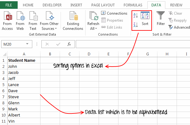
- Next, navigate to the “Data” Tab on the Excel ribbon and click the “A-Z” icon for ascending order sort or the “Z-A” icon for descending sort.
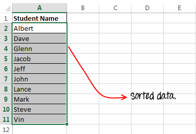
Sorting data table with multiple columns using this method:
If you have a list with two columns like “Student Name” and “Roll number”. And you have to alphabetize this list based on “Student Names”. Then you should use the “Sort” button instead of the “A-Z” and “Z-A” buttons.
The sort button gives you more control over how you want the list to be sorted. It allows you to select only one column to be sorted, it takes care of your table headers and it can also sort your data on the basis of text font or color.
Follow the below steps to use this method:
- First of all, select the table to be alphabetized.
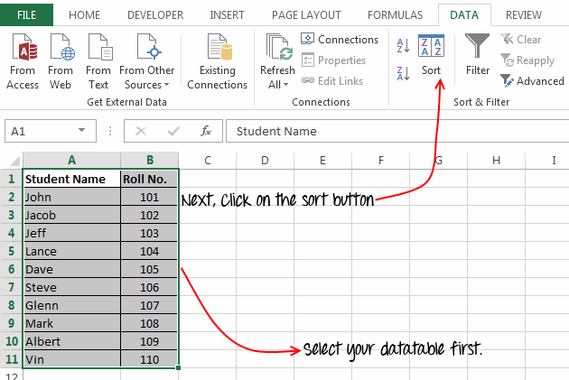
- After this click the “Sort” button, on the “Data” tab.
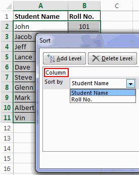
- This will open a “Sort” dialog box, in the ‘Column’ dropdown select the column based on which you want to alphabetize your data.
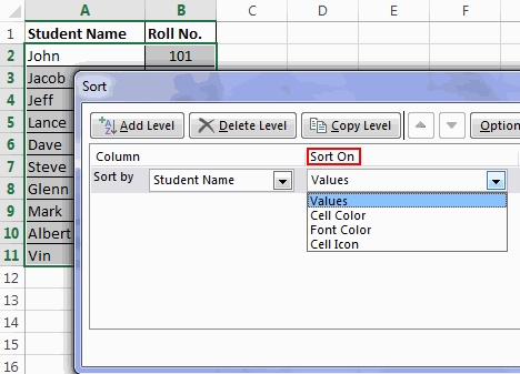
- In the ‘Sort On’ dropdown select the ‘values’ option. Using ‘Sort On’ dropdown you can sort your data based on cell colour, font colour or cell icons.
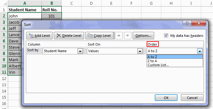
- In the ‘Order’ field select “A-Z” for Ascending sort or “Z-A” for descending sort. If your data is without a header row then uncheck the ‘My data has headers’ checkbox, otherwise, leave it checked.
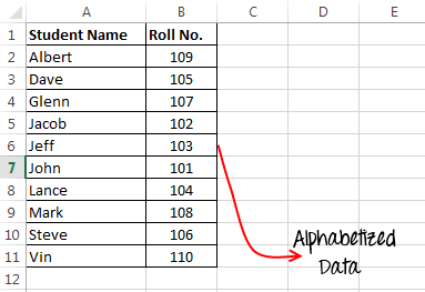
- Finally, click on the ‘Ok’ button and your data is sorted.
Notice that the names are sorted but the corresponding roll numbers have not changed, so the data is still reliable.
Method 2 – Alphabetizing a column using shortcut keys
If you are someone who loves to use the keyboard more than doing the same tasks with a mouse, then here I will share a list of shortcut keys that will be useful for you while sorting columns in excel.
| Keys | Description |
|---|---|
| Alt + D, S | This will open the Sort menu. |
| Alt + H, S, S | This will simulate the click event of “A-Z” icon on the ribbon. (Ascending Sort) |
| Alt + H, S, O | This will simulate the click event of “Z-A” icon on the ribbon. (Descending Sort) |
Note before using these shortcuts make sure that you have already selected your data table.
Method 3 – Sort a list using Excel formula:
In this method, we will use excel formulas to alphabetize a list. The two formulas that we are going to use are COUNTIF and VLOOKUP.
Many of you would be thinking that “how we can sort a list using a CountIf function?” The trick behind this is, we can use the COUNTIF function to count values based on the given criteria.
For example: Suppose we have a list with some alphabets 'o, l, n, m, p, q' in a range A1:A6. Now if we use a formula as:
=COUNTIF("A1:A6",">o")The result would be 3 because only three alphabets (l, m, n) come before 'o'. This clearly indicates that the COUNTIF function if used properly can give us sorting orders.
Let’s use this concept in our previous example.
First of all, we will a temporary column named “Sorting order” to our existing table. After this, we will use a formula =COUNTIF($B$2:$B$11,"<="&B2) for the first student.
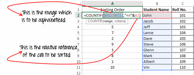
And then we will drag this formula to fill it in the entire range.
This formula gives the sorting order of each of the items in the list. Now, we just have to arrange the data based on the sorting order and for this, we will use a VLOOKUP function.
=VLOOKUP(<sort number>,A:B,2,0)Here ‘sort number’ signifies the numbers in ascending order from 1-10. For descending order sort the numbers should be from 10-1.
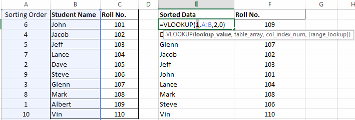
Similarly, for the second and third items, you can use the formula as :
=VLOOKUP(2,A:B,2,0)and
=VLOOKUP(3,A:B,2,0)After applying this VlookUp formula the list gets alphabetized.
Tip: Instead of manually entering the 1-10 in the above formula, you can also use the row function to ease your task. Row() gives you the row number of the current cell.
So, with the use of the row function the formula would be:
=VLOOKUP(ROW()-1,A:B,2,0)Thanks to Chandoo for explaining this method so nicely. You can also find the same tutorial here.
Method 4 – How to alphabetize using Excel Macro
Here is another method for sorting your data, this method can be used if you are looking for alphabetizing your data using a macro.
So here is the macro:
Sub Alphabetize_Range()
Dim fromRow As Integer
Dim toRow As Integer
fromRow = 1
toRow = ActiveSheet.UsedRange.rows.Count
 ActiveSheet.rows(fromRow & ":" & toRow).Sort Key1:=ActiveSheet.Range("A:A"), _
 Order1:=xlAscending, Header:=xlYes, OrderCustom:=1, _
 MatchCase:=False, Orientation:=xlTopToBottom
MsgBox "Your data has been sorted!"
End Sub
Please note that you need to do some customizations in the above macro before using it. Following are the changes:
- If your data is not starting from 1st row then change the
fromRow = 1 - If you need to explicitly specify the row till which sorting should occur then change
toRow = ActiveSheet.UsedRange.rows.Count - This macro sorts the data on the basis of Range "A:A", but you can change it by changing
Sort Key1:=ActiveSheet.Range("A:A")argument. - Change '
Order1:=xlAscending' to 'Order1:=xlDescending' for descending sort. - If your table doesn’t have a header row then change
Header:=xlYestoHeader:=xlNo
So, this was all about how to alphabetize in excel. Do share your thoughts about this topic.
Recommended Reading: How to create a Checkbox in excel


