Excel AND Function – How To Use

The AND function in Excel is a logical function that checks whether all arguments fed into the function are TRUE and returns "TRUE" if all arguments are TRUE. This implies that even one unmet condition will return "FALSE" as the result.

Making its way into Excel in 2003, the AND function serves little functioning on its own.; though it is helpful to evaluate multiple conditions at a time and ascertain if all of them are met. It comes well handy in financial analysis and serves as a better tool in combination with other functions.

This tutorial will guide you on the scenarios where the AND function can be helpful in Excel.

Syntax

The syntax of the AND function is as follows:

Arguments:

logical1 – The first condition to be tested.
logical2 – The second condition to be tested. Entering this argument is optional.

Important Characteristics of AND Function in Excel

• AND function can evaluate up to 255 conditions.
• The result returned with the correct parameters can either be "TRUE" or "FALSE".
• If the argument is 0 (numeric), the result will be "FALSE", similarly 1 is treated as "TRUE".
• If no logical values are found in the formula, the function returns a #VALUE! error.
• If the formula has any typos or misspelling, the function returns a #NAME?
• The arguments can be numbers, cell references, defined names, formulas, functions, or text.

Examples of AND Function

We're going to see a few simple examples of the AND function to understand the works.

Example 1 – AND Function With a Single Parameter

AND function can be used with a single Boolean parameter or any expression that results in a Boolean value.

The formula simply would be:

The function evaluates the condition to be logically either TRUE or FALSE and returns the relevant result. Here we have fed only one logical condition into the function, let's move on to doubling that.

Example 2 – AND Function With Two or More Parameters

Now we will use AND function with two Boolean parameters/expressions that result in a Boolean value.

The function makes the selection based on the fulfillment of multiple conditions very easy. We'll show you how through this example.

We have a list of students. The purpose is to select students to shortlist them for the position of school prefect. Prefects are only selected if they fulfill the following criteria:

1. They have previously been a class monitor. (column C)
2. They have a decent record of not being latecomers. (column D)

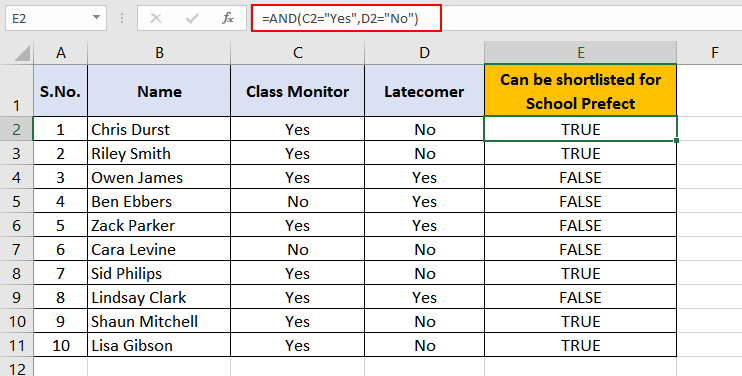
Fulfillment of both conditions will have the students shortlisted for school prefect. We have applied the following formula to make this process easier:

We have passed both the required conditions into the AND function;

• the value in cell C2 must be "Yes"
• the value in cell D2 must be "No"

to bring back the result as "TRUE" in order for the student to be shortlisted.

Case 1 – When Both Parameters Evaluate to TRUE

As for student 1, the AND function will check cell C2 for "Yes" and then cell D2 for "No". Since both conditions are TRUE hence the AND function returns "TRUE" as result. So, "Chris Durst" will be shortlisted as a school prefect.

Case 2 – When Both Parameters Evaluate to FALSE

Student 4 doesn't fulfill both the conditions, the value in cell C5 is "No" and the value in cell D5 is "Yes" and therefore the result is "FALSE". So, "Ben Ebbers" does not qualify for shortlisting as a school prefect.

Case 3 – When One Parameter is TRUE, the Other is FALSE

Student 5 has been a class monitor before but is also a latecomer. The value in cell C6 is "Yes" and the value in cell D6 is also "Yes" and the result is "FALSE". So "Zack Parker" does not qualify for shortlisting as a school prefect.

Note how the AND function evaluates all expressions to return a single Boolean value as the result. In this case, even though the first logical condition (C6="Yes") is met, the function returns "FALSE". This tells us that the AND function will only result in TRUE when all the supplied parameters/expressions evaluate to TRUE. If any expression returns FALSE [(D6="No") in this case], the result of the AND function will be FALSE.

The same can be said for student 6; the first condition (C7="Yes") is not met while the second (D7="No") is. This has also resulted in "FALSE" by the function.

Example 3 – Use of AND Function with IF Function

The role of an IF function is to return a value based on a stated condition. IF functions can be nested within each other to develop formulas for handling complex logic.

Instead of having several nested IF functions to test multiple conditions, the AND function can be nested within the IF function to get a similar customized result.

Carrying forward the example from above, we will show you how the functions work together.

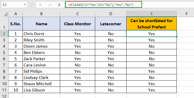
The advantage here of using the AND function within the IF function is that we can get:

• "Yes" instead of "TRUE" and
• "No" instead of "FALSE"

as the result.

We have achieved this by the following formula:

Here, the AND function takes its role first, looks up cell C2 for "Yes" and cell D2 for "No". If the AND function finds both the conditions are met it returns "TRUE" otherwise "FALSE". This result is then passed onto the IF function where the corresponding value for TRUE is "Yes" and for FALSE the value is "No". Since for the first record, both the conditions meet hence the IF function returns "Yes" as the result.

Example 4 – AND Function for finding a value in-between values

Since Excel doesn't have a BETWEEN function, we'll have to tweak the AND function and IF function to find a given value between two values. Luckily, it's not hard at all and is much similar to what we saw above; we will nest the AND function in the IF function. We will show you how to achieve this in the form of:

• Numbers,
• Dates, and
• Text.

This calls for an example.

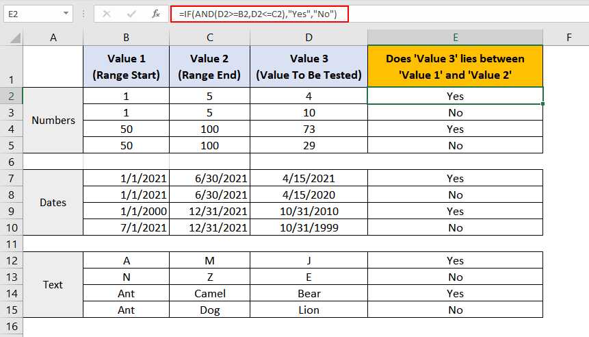
Our aim is to find whether the values in column D are between the values in column B and column C. We brought the AND and IF functions to work like so:

Here, the AND function checks whether the value 4 is greater than or equal to the value 1, which evaluates to "TRUE". Next, the AND function checks if 4 is less than or equal to 5, which also evaluates to "TRUE".

The AND function has done its work, the result is "TRUE" and now it's the IF function's turn. The IF function is written in such a way that it returns "Yes" for a "TRUE" and "No" for a "FALSE". Since in the first case, the AND function has resulted in a "TRUE" value hence the IF displays "Yes".

In this way, the other values are checked to lie between Value 1 and Value 2.

For the "Text" entries, the function performs the search alphabetically; Bear lies between Ant and Camel, Lion does not lie between Ant and Dog. It's true on paper, however weird that may sound.

Example 5 – Use of AND Function in Array Form

The AND function can also be used to evaluate a range of cells and determine whether the condition specified, is met in all of the cells in the range. Let's try to understand this with an example.

In this example, we have a list of students along with their scores. Our objective is to check and see if all the students on the list have got a score of 70 or more.

To accomplish this, we can make use of the AND function in array form as:

Note: This is an array formula and must be entered with Ctrl + Shift + Enter keys, except in Excel 365.

In the above formula, we are asking the AND function to take each cell in the given range i.e. B2:B11, and check if the values in each cell are greater than 70. If all the cells have a value greater than 70, the function returns TRUE otherwise it returns FALSE.

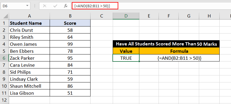
Similarly, we can also check if all the students on the list have scored 50 or more with the following formula:

Note: This is an array formula and must be entered with Ctrl + Shift + Enter keys, except in Excel 365.

Since all the cells in the range B2:B11 have a value greater than 50, hence the result is TRUE.

"And" that was all folks! We hope you learned the basics and complexities of the AND function in good detail. We will have the workings of another Excel function coming for you soon. Forever Excel-sior!