Excel ISERROR Function – How To Use

The Excel ISERROR function checks whether a value is an error. The function only returns TRUE upon finding an error and returns FALSE for all other values.

ISERROR, which literally means 'Is error?', tests all types of Excel errors. Making its entry into the Excel world in 2003, ISERROR comes from a group of IS functions that results in TRUE or FALSE. The syntax of the ISERROR function is just one value argument (like all the other members from the IS functions family). Let's have a look.

Syntax

The syntax of the ISERROR function is as follows:

Arguments:

value – The value or expression that needs to be tested for errors.

Important Characteristics of ISERROR Function in Excel

• The ISERROR function deals with all formula errors in Excel, the function returns TRUE when it finds an error, otherwise, it returns FALSE.
• ISERROR is most commonly used with the IF function to find and handle errors.
• In Excel 2007 or higher, you can use the IFERROR function instead of using ISERROR with the IF function to handle errors.

Examples of ISERROR Function

Let's have a look at the basic work of ISERROR before we go into expanding its functionality.

Example 1 – Simple ISERROR function

The ISERROR function in its plainest form would look something like this:

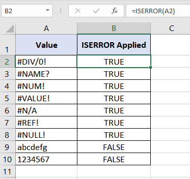
Here, column A is listed with all possible Excel errors. We are using the ISERROR function at its simplest to check column A for errors:

The ISERROR function finds an error in "A2" and returns "TRUE". The same goes with cells "A3" to "A8" all of which contain different error types. ISERROR results in FALSE upon finding no errors in "A9" and "A10". This shows that the ISERROR function traps all types of formula errors.

Now that the ISERROR function has made its introduction, let's see what else it can do.

Example 2 – ISERROR function with IF function

The IF function in Exel is the easiest way to get most functions to be more user-oriented. The IF function checks if a given condition is met or not and returns the value set for either case. Let's say we are in favor of attaining these custom values and not TRUE/FALSE. Using the ISERROR and IF functions together will help us with that. Let's refer to an example.

Here, we have a dataset from 10 types of T-shirts. The data we have regarding the T-shirts are the total sales for each design type and its unit price. Our objective is to calculate the units sold of each type (dividing sales by price).

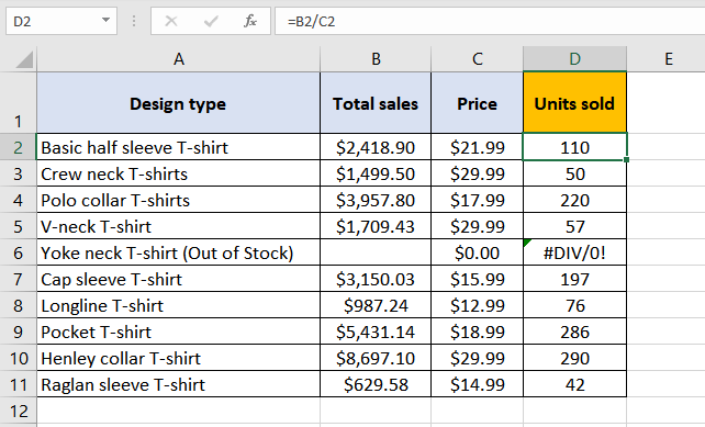
The #DIV/0 errors have occurred due to some missing prices of products. These don't give our worksheet a nice look. Let's try to present these errors in a better way.

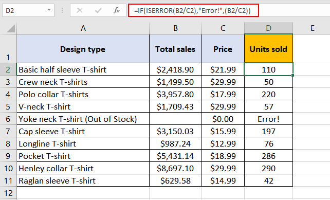
Using the following formula, we have swapped the #DIV/0 errors out with a custom value "Error!":

Starting with the "Basic half sleeve T-shirt" in cell B2, the ISERROR function checks "B2/C2" for errors. Since, in this case, no errors are found; ISERROR's result is FALSE. For a FALSE result, the IF function is set to display the result of "B2/C2" (which is 2,418.90/21.99 = "110").

Now, let's analyze cell D6. Since the 'Yoke neck T-shirt' is out of stock so its price and total sales numbers are not available. Here, the ISERROR function checks "B6/C6" for an error and finds a #DIV/0 error (0/0 = #DIV/0), so ISERROR returns a TRUE. For a TRUE result, instead of showing the #DIV/0 error, the IF function is set to display the supplied value "Error!".

Example 3 – ISERROR function with the SUM function

We can use the SUM and ISERROR functions to count the total number of errors in a range of cells.

Let's take a look at Example 1.

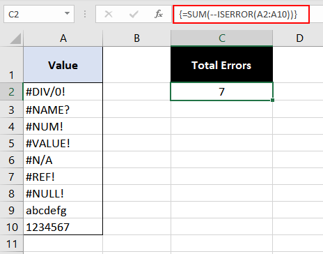
The formula used is:

Note: This is an array formula and must be entered with Ctrl + Shift + Enter keys, except in Excel 365.

The ISERROR function applied to the range on its own will split into the supplied cell range and give the result of each cell individually like this:

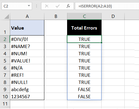
Upon finding errors from "A2" to "A8" and no errors in "A9" and "A10", the result of the ISERROR function is TRUE, TRUE, TRUE, TRUE, TRUE, TRUE, TRUE, FALSE, FALSE. The double unary operator in the formula converts TRUE and FALSE into their respective numeric values as 1 and 0. The result now is 1, 1, 1, 1, 1, 1, 1, 0, 0. The SUM function takes ISERROR's result, adds it up, and displays "7" as the final result.

ISERROR vs IFERROR Function

IFERROR is like having the ISERROR and IF functions combined in one to give us lesser work to do. Upon finding an error, the IFERROR function returns a custom value otherwise it returns the value of the expression itself.

Sounds like a winning situation. Let's see if it is.

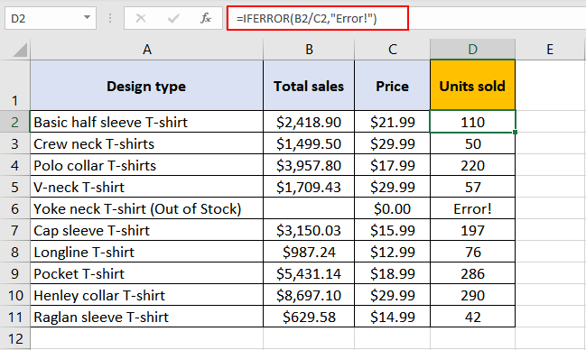
Here we have used the data from Example 2 but switched IF and ISERROR functions for the IFERROR function alone. Here's the formula we used:

How does it work?

The IFERROR function checks "B2/C2" for errors, it finds the expression error-free and returns the result of the expression as it is (which is "110"). Coming down to the #DIV/0 error in cell D6. Since B6/C6 results in a #DIV/0 error, so the IFERROR traps the error and returns a custom value "Error!" which it displays as the final result.

Now it looks like a winning situation too; we have attained exactly the same results as with the ISERROR and IF functions combined. Also, note how simple and easy to read this formula is in comparison to Example 2.

How to Choose Between ISERROR & IFERROR

Both functions cover all Excel kinds of formula errors.

The ISERROR function by itself will result in TRUE/FALSE and hence requires the IF function to return a more meaningful output.

The IFERROR function on the other hand returns a custom output when the supplied expression results in an error. It is simpler than using ISERROR and IF together.

Another point worth noting is – IFERROR function automatically assumes that you will always want the result of the expression if your expression doesn't have any errors. ISERROR, on the other hand, gives you a boolean value (either TRUE or a FALSE), and when combined with the IF function, it allows you to have more control over the result in both outcomes.

ISERROR vs ISERR Function

Why has there been so much emphasis on ISERROR covering all Excel errors? There are some functions that by design deal with lesser errors.

Little brother of ISERROR, ISERR deals with all Excel errors except the #N/A error. ISERR function returns TRUE if any error (except the #N/A error) is detected and FALSE for #N/A errors and all other values.

This may seem like a shortfall but could be handy where #N/A errors don't need to be accounted for by the function and need to stand out as missing information instead of other errors. Let's look into this with an example.

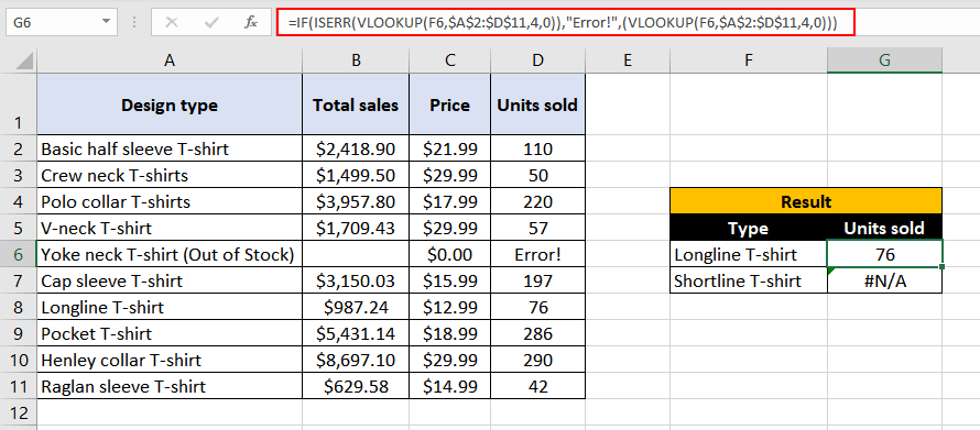
We are trying to find the units sold of certain shirt types with this formula:

That seems like a lot to take in but that's why we're here.

In the first case, VLOOKUP's job is to find the value mentioned in cell "F6" from the first column of the table "A2:D:11" (the "$" signs are to keep this table constant in the formula). The value to return is in the "4^th" column. "0" in the formula means that an exact match must be found by VLOOKUP.

This formula finds "Longline T-shirt" in column A, picks up the corresponding value from column D which is a "76". Next, the ISERR function evaluates VLOOKUP's result, which is not an error and so "76" is returned as the final outcome.

In the second instance, VLOOKUP was unable to find "Shortline T-shirt" in column A as it is not listed in our dataset. VLOOKUP returns the #N/A error. The result is passed to ISERR which does not handle #N/A errors and displays the #N/A error. This outcome is favorable in this case as using the ISERR function will account for other errors and deliver "Error!" and #N/A errors will show up to indicate that data is missing.

All things the same, this is what will happen if we replaced ISERR with ISERROR:

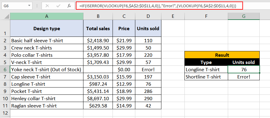
The ISERROR function traps all errors including the #N/A errors. This makes it hard to pinpoint that the error in the second instance is because "Shortline T-shirt" is missing from our set of data. In this instance, it's more helpful to use the ISERR function.

How to Choose Between ISERROR & ISERR

The #N/A error usually comes up with lookup functions so, if the worksheet in question is not working with lookup functions, good chances are that the #N/A error won't pop up to ruin the day. In that case, there isn't a need for dealing with #N/A errors and the ISERR function would be a good pick. In case a #N/A error comes up, it can be handled by correcting the missing data (which is what #N/A errors indicate).

The ISERROR function heroes all Excel errors. It will trap and treat all errors, with the inclusion of the #N/A error, signaling the presence or absence of any errors in the data.

The results of ISERROR and ISERR are in TRUE/FALSE form and both may take help from the IF function to change TRUE/FALSE into more meaningful outputs.

That'll be it for now. By now you may have gotten an idea on how to go about error dealing as annoying as they may be. Reminds us of a joke:

I hate spelling errors.

You mix up two letters and your whole post is urined.

We hope this didn't ruin our whole post.