Excel NOT Function – How To Use

The Excel NOT function is categorized as a logical function. According to MS Excel, "The NOT function changes FALSE to TRUE, or TRUE to FALSE".

What we’re saying is that the function results in the opposite outcome of its fed parameters. The NOT function is beneficial in the cases where we wish to verify if a specific condition was not met.

We see the NOT function going way back to 2003 where it made its place in the Excel world with its other logical function friends.

Syntax

The unfussy syntax of the NOT function is as follows:

Arguments:

logical – The value or condition to be tested.

Important Characteristics of NOT Function in Excel

• NOT function returns either "TRUE" or "FALSE" and can evaluate up to 255 conditions.
• If an argument is the number 0, the result will be "TRUE". Excel processes 0 as FALSE. The NOT function changes FALSE to TRUE.
• If no logical values are found in the formula, the function returns a #VALUE! error.
• If the formula has any typos or misspelling, the function returns a #NAME?
• The arguments can be numbers, cell references, defined names, formulas, functions, or text.

Examples of NOT Function

The talk is better when practically put to the test. So let’s see some examples to understand why the NOT function does the opposite of what it’s told.

Example 1 – Super Duper Basic NOT Function

Riddle time.

Question – What is not TRUE?
Answer: FALSE

Question – What is not FALSE?
Answer: TRUE

See how easy that was? That wasn’t even in Excel language. Working with Boolean parameters, bringing out this function’s ability could not get simpler than this:

We’re making the NOT function’s life too easy. We can make it work harder.

Example 2 – Plain Vanilla Version of NOT Function

Let’s say Gina loves granola. We have granola bars enlisted with allergens that they contain since Gina has a severe peanut allergy.

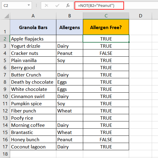
Our objective here is to pick out the bars that contain peanuts so Gina can steer clear of them. That’s achievable with this formula:

What this formula is doing is looking up column B for the word "Peanut". Since the command is for the cell to not contain "Peanut", if the word "Peanut" is found, the result would be "FALSE". If it is not found, the result will be "TRUE".

• Cell "C2" asks cell "B2" ‘NOT Peanut?’. "B2" is blank, it’s TRUE, "B2" is ‘NOT Peanut’.
• Cell "C4" asks cell "B4" ‘NOT Peanut?’. "B4" is "Peanut", it’s FALSE.

Gina has to keep away from the "FALSE" results. Luckily, she has a lot of peanut-free options.

Example 3 – Use of NOT Function with IF Function

The role of an IF function is to return a value based on a stated condition. Bringing forward the example from above, we take a look at how the 2 functions go together.

The plus point here of using the NOT function within the IF function is that we can get:

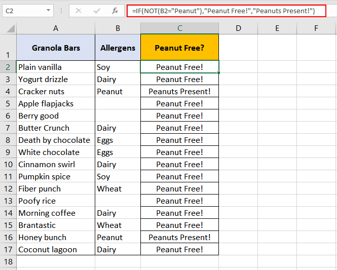
• "Peanut Free!" instead of "TRUE" and
• "Peanuts Present!" instead of "FALSE"

as a result.

We use the following formula:

Firstly, the NOT function starts its work, looks up the "B2" cell to check whether it contains "Peanut". NOT function finds "B2" cell blank, which implies "B2" is "NOT" equal to "Peanut". And thus, the result of the NOT function is "TRUE".

The result is passed onto the IF function where the corresponding value for TRUE is "Peanut Free!". Hence the IF function returns "Peanut Free!" as a result.

Example 4 – NOT "X" OR "Y"

The OR function can be used to evaluate an array of values and determine whether the condition specified is met in at least one value or not. Let’s carry forward the example above.

It turns out Gina isn’t as lucky as we thought; she is also allergic to soy! Which means her favorite granola bars need to be peanut and soy-free. Let’s help her.

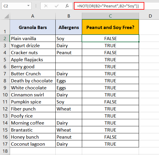
We need to find granola bars that do not contain peanuts or soy. To find these two allergens, the formula we’ve applied is:

The OR function has been asked to check cells from B2 to B17 and see whether they contain

• "Peanut" or
• "Soy".

The OR function finds "B2" contains "Soy". Since one argument of the function is fulfilled, the result is "TRUE". This result is passed onto the NOT function.

The NOT function flips "TRUE" to "FALSE".

The core purpose of having the NOT function here anyway is to find out whether "B2" is NOT "Peanut" OR "Soy". So as the greater picture, the result is also "FALSE" and that is the result returned in C2.

IF NOT "x" OR "y"

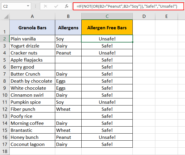
To attain the same customized result seen in Example 3, we can easily incorporate the IF function by this formula:

The results are in column C. Adding the IF function has customized the results into:

• "Safe!" instead of "TRUE" and
• "Unsafe!" instead of "FALSE".

That would be it. NOT the last you hear from us. Since we talked so much about granola bars, you know what else you can do on Excel?

You can make a pie chart of your favorite bars.

And a bar graph of your favorite pies.

We’ll be back with more… functions, not jokes.