The term transpose literally means swapping rows and columns. And similarly transpose function in excel flips rows into columns and vice-versa. Transpose is an array function i.e. it can only be applied on a range of cells. And today in this post I will be guiding you on how to use transpose functionality in excel.
What are Array Functions and why transpose is an Array function?
Array functions are different from normal functions as they deal with block of cells instead of a single cell. Sometimes array functions are also called CSE functions, because these functions can only be entered by pressing “Ctrl + Shift + Enter” keys at the same time. Array functions are enclosed by curly braces ‘{}’.
Transpose is also an array function because it is applied on a block of cells. It is absurd if you are applying a transpose function on a single cell, as flipping a row into a cell doesn’t makes sense.
Method 1: To apply transpose function using Paste Special option:
Applying transpose using the paste special option is an easy way to perform transpose function in a much easier way. Follow the below steps to do this:
1. Select and copy the range of cells that you want to transpose.
2. Next, Right Click on the area where you want to paste the transposed result.
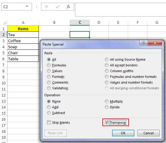
3. Now click the ‘Paste Special’ option, this will open the ‘Paste Special’ window.
4. In the ‘Paste Special’ window check the option that says ‘Transpose’ and hit the ‘OK’ button.
5. This will transpose your data and will paste it in the selected cell.
Method 2: To apply transpose function using formula:
Transpose functionality of excel can be implemented in much better way using the transpose formula that excel supports. I have said this method better because in this way the results are dynamically generated from the original range unlike the above method. So, if after using this method your original data gets changed, then the change will be reflected in the transposed data as well. Follow the below steps to use this method:
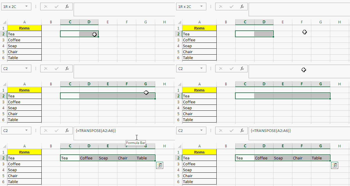
1. First of all select the range where you want to transpose your data.
2. Next, while keeping the block of cells selected enter the formula in the above formula bar.
=transpose(range1)
The ‘range1’ argument signifies the range of cells that you want to transpose.
3. After entering the formula, press the keys “Ctrl + Shift + Enter” this will enclose the formula into curly braces.
{=transpose(range1)}
4. This will apply the formula on the selected range. And you will be able to see the transposed cells in the selected block of cells.
Note 1: After applying this formula you cannot individually edit or delete any of the cells from the transposed range.
Note 2: After applying this formula if you change any one of the original cell then this change will also be reflected in the corresponding transposed cell.
This was all about Transpose Function in Excel. Do let us know if you face any issues while applying it.


