How to Add a Total Row in Excel Table (2 Easy Ways)

In this tutorial, you will learn how to add a Total Row to an Excel table. If you’re wondering what Total Rows and Excel Tables are, don't worry. We’re going to tackle them one by one but before that, let's get some background.

Excel 2007 came up with a feature called "Excel Tables". Although Excel Table is an overly generic term, they provide some handy features to view and report data in tabular format. Apart from the countless features of the Excel table, they also give you an out-of-box ability to have a Total Row added to the bottom of your table.

The Total Row will not just present itself with a total figure, but the entire row can be used to summarize data by sum, average, count, minimum, maximum, and many other amazing aggregate functions. Before going any further into today's topic, let’s address the elephant in the room – the Excel table.

Table of Contents

What is an Excel Table?

If you are also under the common confusion that any table in an Excel file is an Excel table, let’s begin by clearing that up for you. A table made up of rows, columns, and data is a dataset. You will actually have to convert the dataset into an Excel table to be able to use its many features.

While a dataset will give the benefit of being organized, an Excel table can take that further, making the data dynamic (adjusting the range with added or deleted data), pre-styled, and easier to analyze & summarize through its several useful and convenient features. One of such convenient features of an Excel Table is the Total Row, which gives you the summary of calculations for each column with different data aggregation functions.

This helps you to have an instant overview of the data without much effort. Now, let's see how to convert your datasets into an Excel Table.

Converting Dataset into an Excel Table

Let’s suppose the plain dataset below is what you have to start with. Follow along to covert this dataset into an Excel Table:

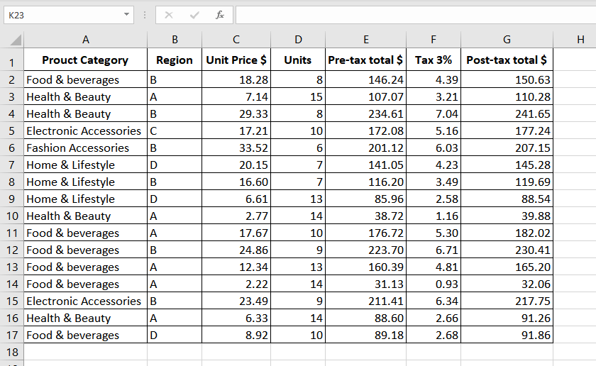
Select any cell in the table.
From the Home tab, in the Styles group, click Format as Table. You will see a menu from where you can select the style for the Excel Table.

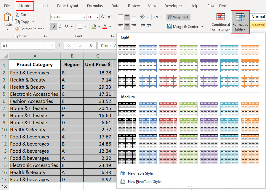
From the Home tab, in the Styles group, click Format as Table

Alternatively, you can use the keyboard shortcut Ctrl + T to create an Excel Table. This option will automatically set the style to Table Style Medium 2, Blue, which can be changed later.
Upon selecting the style, you will get a Create Table dialog box asking the range of the table. This is why you need to select a cell in the table in Step 1, so Excel can estimate the range of the table.

Create Table dialog box asking the range of the table

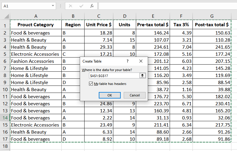
The marching-ants line denotes the range Excel guesses for the table. Make the adjustments here in the dialog box if Excel’s guess is not right.
If your table already contains headers, make sure the My table has headers checkbox is checked. Otherwise, this feature will assume no headers in the table and will create a new header row above the table.
Click OK, and your Excel Table is ready!

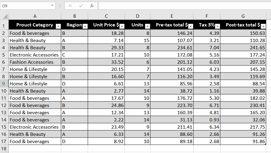
Benefits of Excel Tables

Converting our dataset into an Excel table has the following benefits:

The biggest advantage of tables is that they are dynamic in nature, which means that they can expand as the new data is added or can shink when the data is deleted.
Converting the dataset into an Excel table gives you the option of sorting and filtering in every column of the table.
Provides a preset style that can be changed.
Opens up several handy features like calculated columns, structured references, etc.
One of these countless features is the ability to have Total Row for data summarization, and this is what we are going to see next.

Recommended Reading: Everything About Named Ranges in Excel

Adding a Total Row to an Excel Table

Adding a Total Row is as uncomplicated as making the table itself, and there are 2 easy ways of doing this. One from right-click context menu on the table and the other from the Design tab in the ribbon. Let’s walk you through both.

Method 1 – Adding Total Row from the Right-click Context Menu

Right-click any cell of the Excel table. This will display the right-click context menu.

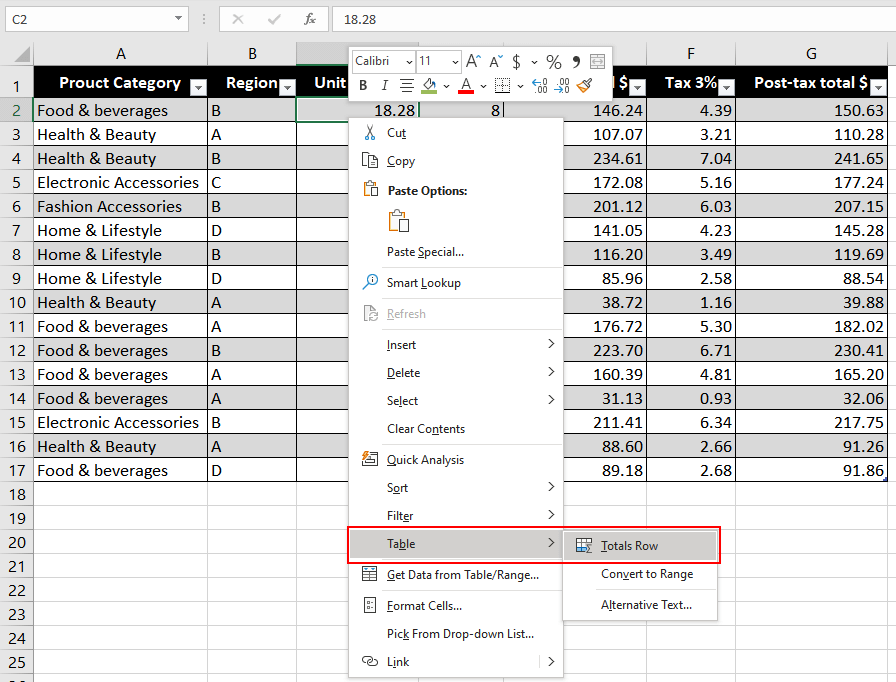
In the menu, navigate to Table, and from the following sub-menu, select Totals Row.

In the menu, navigate to Table, and from the following sub-menu, select Totals Row

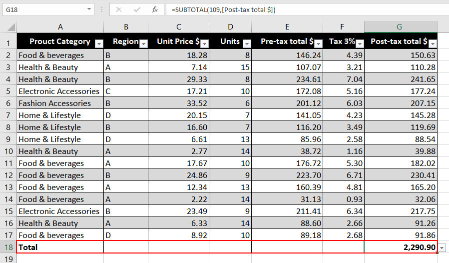
And there it is, the Total Row.

Method 2 – Adding Total Row from the Table Design Tab

Select any cell of the Excel table.

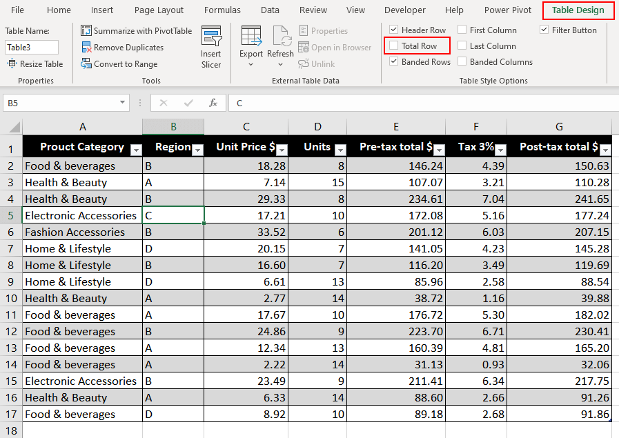
Under the Table Design tab, in the Table Style Options, check the Total Row checkbox.

Under the Table Design tab, in the Table Style Options, check the Total Row checkbox

Equally easy, there is the Total Row.

Pro Tip: The Total Row can be toggled in and out of display by selecting any cell in the Total Row and pressing Ctrl + Shift + T.

Now that you know how to add a Total Row, let’s discover its power.

Customize Totals with the SUBTOTAL function

Once you have added the Total Row, each cell in the row gets its own drop-down list. You can access the drop-down by clicking on the relevant cell, which will display a tiny arrow in a box like the ones in the header row. These drop-down lists provide control over what you would like to see in the Total Row.

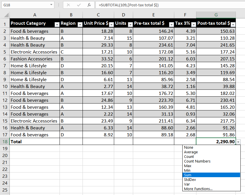
Every option in this list is automatically calculated by the Excel SUBTOTAL function that ignores hidden rows and performs the required task (e.g., calculating and displaying the total or the average value of the column). This is further explained below.

Suppose you want to fetch the average unit price in the Total Row. To do this, inside the Total Row on the Unit Price column, select Avg from the menu.

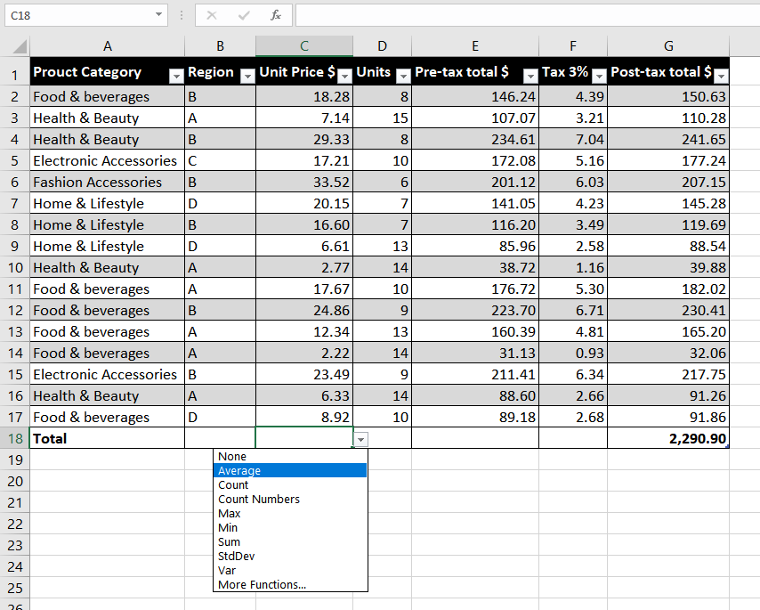
This will display the average unit price in the chosen column.

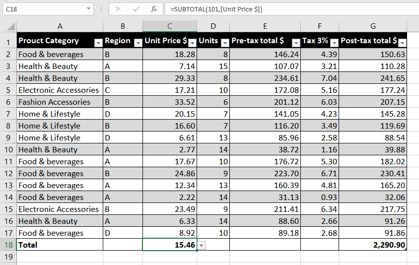
This will display the average unit price in the column

Notice above, with our result selected, the formula in the formula bar. With no work from us here, there is a SUBTOTAL function bringing our desired result for us. Excel automatically uses the SUBTOTAL function to perform the calculation chosen in the drop-down list of the Total Row. 101 in the arguments is a code given to the average calculation. Similarly, 109 is the code for Sum, 103 for Count, 104 for Max, and 105 for Min, etc. The next argument to the SUBTOTAL function is the column header.

Excel uses the SUBTOTAL function instead of the SUM, AVERAGE, or other functions as SUBTOTAL inherently ignores hidden rows and performs multiple calculations. While you can edit the SUBTOTAL function in the formula bar, you can also use the last option from the Total Row drop-down list, which is More Functions.

you can also use the last option from the Total Row drop-down list, which is More Functions

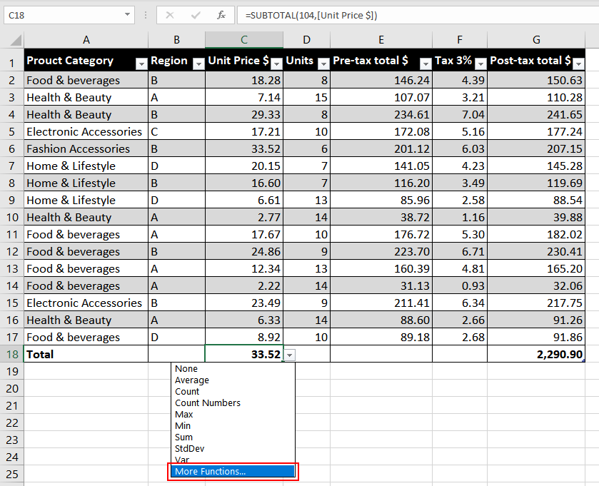
Here you will have a vast choice of functions to choose from to add as a valuable part of your Total Row.

Here you will have a list of functions to choose from to add as a valuable part of your Total Row.

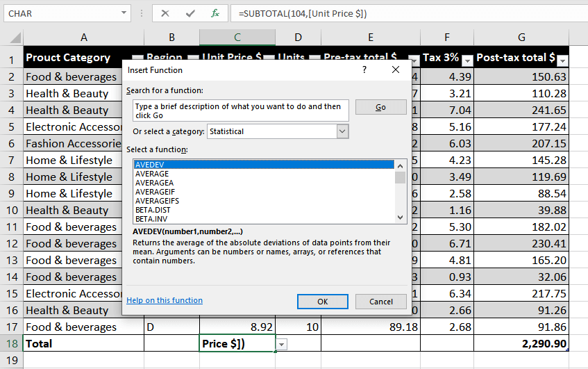
In these ways, you can regulate what you want to see throughout the Total Row of your Excel Table.

And that’s totally the end. We quite hope to have given you an easy grasp of the Total Row and some understanding of how Excel tables work. There’s always more coming from planet Excel; we will keep you enlightened!