Let’s consider we have a long list of duplicate values in a range and our objective is to count only the unique occurrences of each value.
Though this can be a very common requirement in many scenarios but excel doesn’t have any single formula that can directly help us to count unique values in excel inside a range.
In today’s post, we will see 5 different ways of counting unique values in excel.
But, before starting let’s make our goal clear.
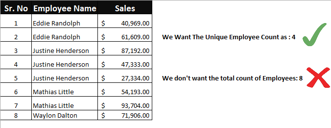
By looking at the above image, we can clearly see that what we mean by counting unique value in excel.
Method – 1: Using SumProduct and CountIF Formula:
The simplest and easiest way to count distinct values in excel is to use SumProduct and CountIF formula.
Following is the generic formula that you can use:
=SUMPRODUCT(1/COUNTIF(data,data))‘data’ – data represents the range that contains the values
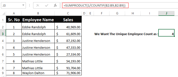
Let’s See How This Formula Works:
This formula consists of two functions combined together. Let’s first understand the role of inner CountIF function.
The CountIF function looks inside the data range (B2:B9) and counts the number of times each value appears in data range.
The result is an array of numbers and in our example it might look something like this: {2;2;3;3;3;2;2;1}.
Next, the results of CountIF formula are used as a divisor with 1 as numerator. This modifies the result of CountIF formula such that; values that only appear once in the array become 1 and the numbers corresponding to duplicate values become fractions corresponding to the multiple.
This means that, if a value appears 4 times in the range then its value will become as 1/4 = 0.25 and value that is present only once will become 1/1 = 1
Finally, the SumProduct formula adds up all the elements in the array and returns the final result.
Read these articles for more details on CountIF Function or SumProduct Function.
The Catch:
This formula woks nicely on a continuous set of values in a range, however if your values contain empty cells, then this formula fails. In such cases the formula throws a ‘divide by zero’ error.
Because, CountIF function generates a ‘0’ for each blank cell and when 1 is divided by 0 it returns a divide by zero error.
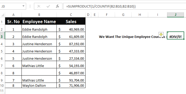
To fix this, you can use the following variant of the above formula that ignores the blank cells:
=SUMPRODUCT(((data<>"")/COUNTIF(data , data &"")))‘data’ – data represents the range that contains the values
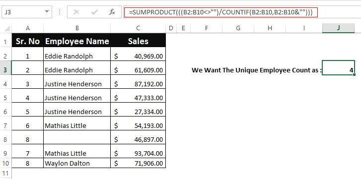
Method – 2: Using SUM, FREQUENCY AND MATCH Array Formula
The formula that we discussed above is good to be used for small ranges. As the range becomes bigger the SUMPRODUCT and COUNTIF formula will become slower and will eventually make your spreadsheets unresponsive while counting unique values inside a range.
So, for larger datasets, you may want to switch to a formula based on the FREQUENCY function.
The generic formula is as follows:
=SUM(IF(FREQUENCY(IF(data<>"", MATCH(data,data,0)),ROW(data)-ROW(firstcell)+1),1))Here, ‘data’ represents the range that contains the values.
And ‘firstcell’ represents the first cell of the range.
Note: This is an array formula so, after writing the formula press ‘Control-Shift-Enter’ and the formula will get surrounded by curly braces as shown below.
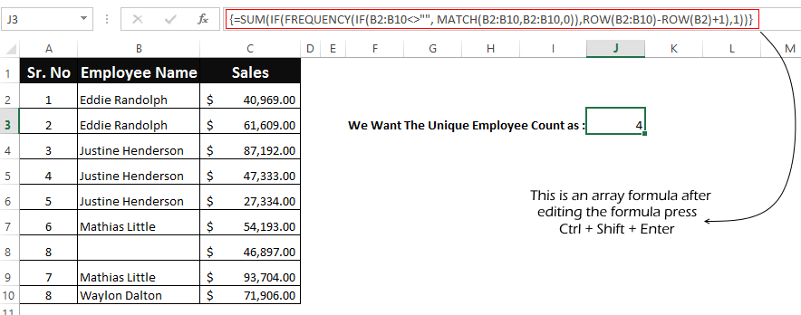
Let’s Try To Understand How This Formula Works:
This formula uses Frequency function to count the unique values, but the problem here is that FREQUENCY function is only designed to work with numbers. So, here our first objective is to convert the values into a set of numbers.
Starting from inside, the MATCH function in this formula gives us the first occurrence or position number of each item that appears in the data range. If there are any values that are duplicate, then MATCH will return only the position of the first occurrence of that value in the data range.
After the MATCH function, there is an IF Statement. The reason IF function is required because MATCH will return a #N/A error for empty cells. So, we are excluding the empty cells with data <> "".
The resulting array contains a set of numbers combined with False for the blank cells. So, in our case the resulting array would be like:
{1;1;3;3;3;6;FALSE;6;9}
This array is fed to the FREQUENCY function which returns how often values occur within the set of data and finally the outer IF function sets each unique value to 1 and duplicate value to FALSE.
And the final result comes out to be 4.
Method – 3: Using PivotTable (Only works in Excel 2013 and above)
The integration of power pivot with excel (known as Data Model), has provided some powerful features to the users. Now pivot tables can also help you to get the distinct counts of unique values in excel.
To do this follow the below steps:
- Navigate to the ‘Insert’ option on the top ribbon and click the ‘PivotTable’ option.

- This will open a ‘PivotTable’ dialog, select the data range and check the checkbox that says ‘Add this data to Data Model’ and finally click ‘Ok’ button.
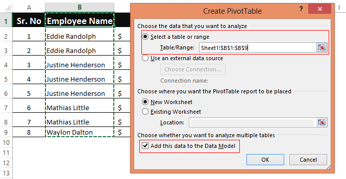
- Build the PivotTable by placing the column that contains data range ‘Values’ and in the ‘Rows’ quadrant as shown below.
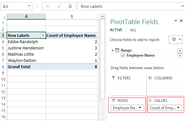
- Doing this will show the total count including the duplicate values, however we only need to get the count of distinct values. So, right click over the Count column and select the ‘Value Field Settings’ option.
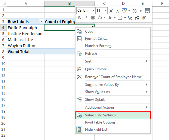
- Next, In the ‘Value Field Settings’ window, select the ‘Distinct Count’ option and click ‘Ok’ button.
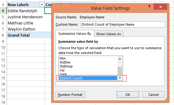
- Doing this will fetch the distinct counts for the values and populate them in the PivotTable.
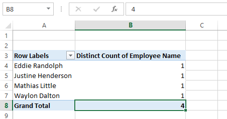
Method – 4: Using SUM and COUNTIF function
This is again an array formula to count distinct values in a range.
=SUM(IF(ISTEXT(range),1/COUNTIF(range, range), ""))Here, ‘range’ represents the range that contains the values.
Note: This is an array formula so, after writing the formula press ‘Control-Shift-Enter’ and the formula will get surrounded by curly braces as shown below.
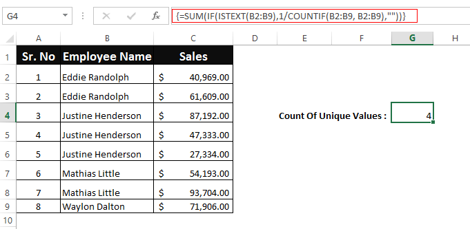
Let’s See How This Formula Works:
In this formula, we have used ISTEXT function. ISTEXT function returns a true for all the values that are text and false for other values.
If the value is a text value, then the COUNTIF function executes and looks inside the data range (B2:B9) and counts the number of times that each value appears in data range.
After this, the result of CountIF function are used as a divisor with 1 as the numerator (same as in first method). This means that, if a value appears 4 times in the range its value will become as 1/4 = 0.25 and when the value is present only once then it becomes 1/1 = 1
Finally, the SUM function computes the sum of all the values and returns the result.
Method 5 – COUNTUNIQUE User Defined Function:
If none of the above options work for you, then you can create your own user defined function (UDF) that can count unique values in excel for you.
Below is the code to write your own UDF that does the same:
Function COUNTUNIQUE(DataRange As Range, CountBlanks As Boolean) As Integer
Dim CellContent As Variant
Dim UniqueValues As New Collection
Application.Volatile
On Error Resume Next
For Each CellContent In DataRange
If CountBlanks = True Or IsEmpty(CellContent) = False Then
UniqueValues.Add CellContent, CStr(CellContent)
End If
Next
COUNTUNIQUE = UniqueValues.Count
End Function
To embed this function in Excel use the following steps:
- Press Alt + F11 key on the Excel, this will open the VBA window.
- On the VBA Window, right click over the ‘Microsoft Excel Objects’ > ‘Insert’ > ‘Module’.

- Clicking the ‘Module’ will open a new module in the Excel. Paste the UDF code in the module window as shown below.
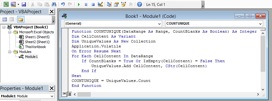
- Finally, save your spreadsheet and the formula is ready to use.
How to Use the UDF:
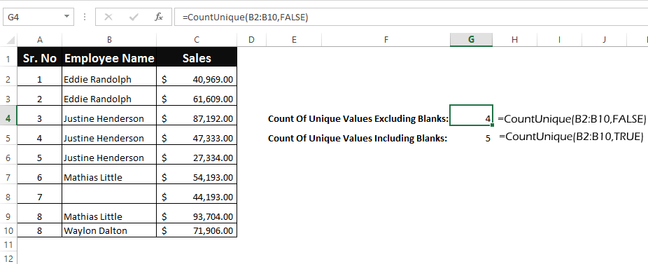
To use the UDF, you can simply type the UDF name ‘CountUnique’ like a normal excel function.
=COUNTUNIQUE(data_range, count_blanks)‘data_range’ – represents the range that contains the values.
‘count_blanks’ – is a boolean parameter that can have two values true or false. If you set this parameter as true then it will count the blank rows as unique. By setting this parameter to false the UDF will exclude the blank rows.
So, these were all the methods that can help you to count unique value in excel. Do let us know your own methods or tricks to do the same.


