How to Highlight Every Other Row in Excel (3 Easy Ways)

Cells can be highlighted in Excel using the Fill Color option. Rows and columns are no different. As it always stands, dealing with a small dataset is no problem at all but the problem gets bigger with the bigger datasets.

We just want systematic selection and highlighting. It's not too much to ask for. If you're cracking your knuckles on how to make something so simple work Excel-ly, we have this detailed guide just so you can spare your knuckles (and of course so you can highlight alternate rows).

Our objective in this tutorial is to highlight every other row in our dataset and we have few good ways of getting that done. Let's get highlighting! Alternately.

Method #1 – Using Manual Approach

Other than holding down the Ctrl key and clicking every other row, there's another manual method that involves filtering and the ISEVEN function. The ISEVEN function returns TRUE if the specified number is even.

The process starts with numbering all the rows in a separate column. Then using the ISEVEN function in another column which will return TRUE for alternate rows. By filtering, all TRUEs (or FALSEs) can be grouped and highlighted. After the filter is removed, every alternate column will be highlighted. The two new test columns involving the numbering and the ISEVEN function can then be deleted. Now let's show you the detailed steps.

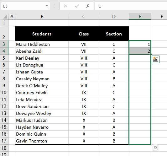
• Along the last column in your dataset, type 1 in the first row and 2 in the next row. Select both these cells, click and drag to fill the column with consecutive numbering.

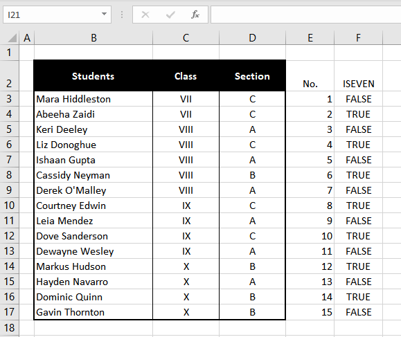
• In the next column, enter the ISEVEN function:
  =ISEVEN(E3)

• For ease of referring, we will name these two columns "No." and "ISEVEN".

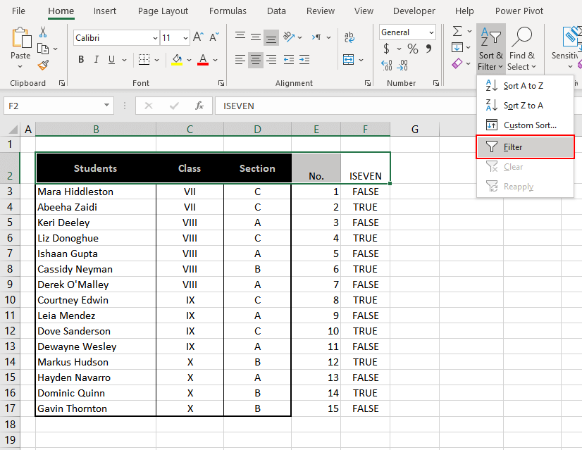
• From the Home tab, in the Editing section, click the Sort & Filter From the drop-down menu, select Filter. Alternatively, use the keyboard shortcut Ctrl + Shift + L to turn on filtering for the table.

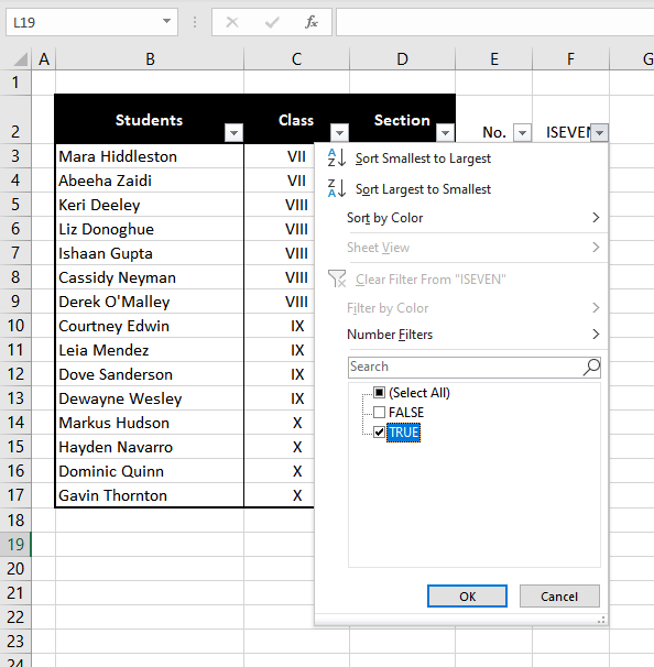
• By clicking on the little arrow above the ISEVEN column, uncheck the Select All checkbox, then filter the column to any one group (either TRUE or FALSE).

• Select the filtered data and highlight it.

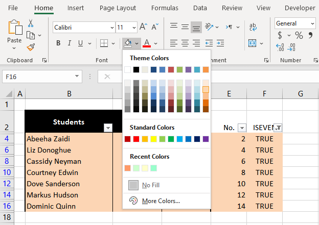
• Now clear the Filter from the "ISEVEN" column. You can then also remove the filters by clicking anywhere in the table and pressing Ctrl + Shift + L or selecting the Filter option again from the ribbon menu.

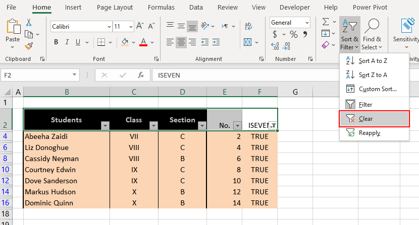
• Expanding back to the original dataset shows you that every other row is highlighted.

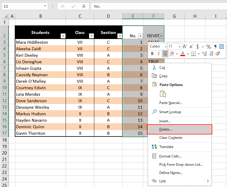
• Select both the test columns (columns E and F) and delete them.

Similarly, instead of having a separate column for numbering the rows, the ROW function can be fed into the ISEVEN function like so:

This will work in the same way as the steps mentioned above. This formula will basically work as "is this row an even-numbered row?" and return TRUE or FALSE.

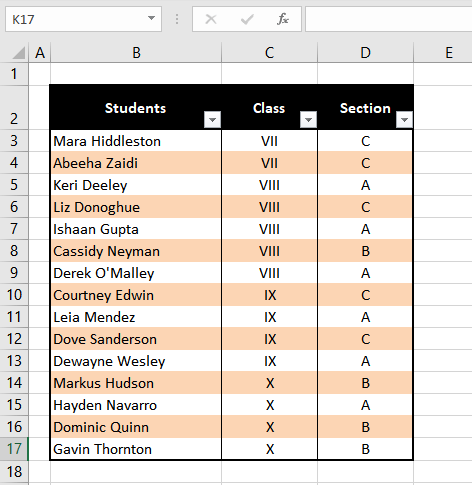
Here onwards, the table can be filtered, grouped, highlighted, unfiltered and the helper column deleted like the steps from above.

Recommended Reading: How To Rotate Cell Text In Excel

Method #2 – Using Conditional Formatting

Now we can take things to the next level and make use of Excel's conditional formatting feature to highlight alternate rows. In this process, we are going to conditionally format our data using a formula based on the  ROW function such that the formula returns TRUE for every alternate row.

To accomplish this we can use the formula that we saw in the section above or we can build another formula based on the MOD and ROW functions together. The MOD function returns the remainder after a number is divided by another number (e.g. number 5, divided by 2, MOD will return the remainder 1).

Sounds easy, doesn't it? It is when you know what to do so here is what to do:

• Select the dataset requiring highlighted rows.
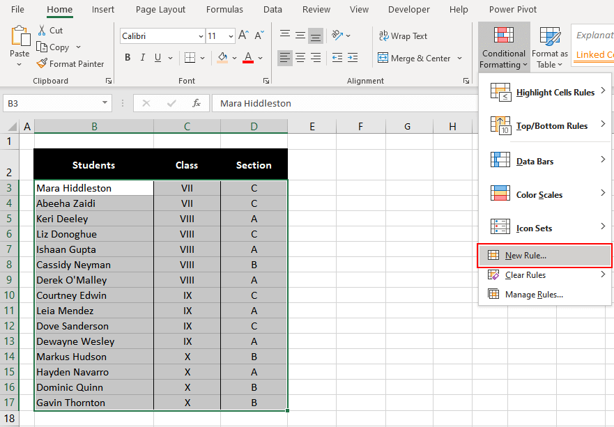
• From the Home tab, in the Styles section, click the Conditional Formatting From the drop-down menu, select the New Rule option. This will open the New Formatting Rule window.

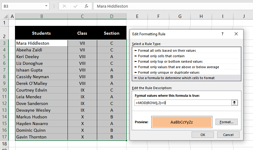
• From the Select a Rule Type: section, select Use a formula to determine which cells to format. This option will allow us to use the MOD and ROW functions to conditionally format our selected data.
• In the formula bar, enter any one of the formulas below (both formulas will return the same result):

or

• Next, click the Format… button below to launch the Format Cells window.

• We are aiming to highlight the rows so we will go to the Fill tab and select the color for highlighting.

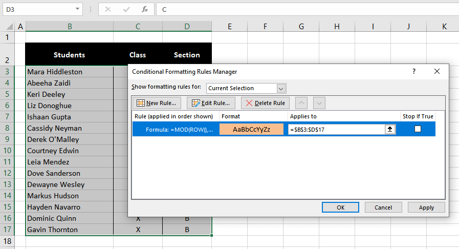
• Then click OK in the Format Cells window and also the New Formatting Rule window to apply the conditional format.

Presenting successfully highlighted alternate rows:

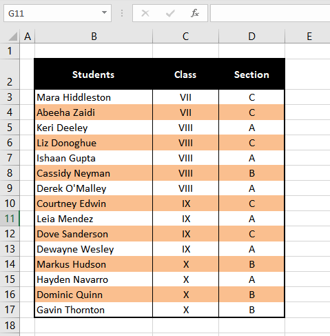
Job well done!

Highlighting Every 3rd, 4th, or nth Row With Conditional Formatting

In the above section, we saw how to shade every other row using conditional formatting in Excel.

What if we wish to shade every 3rd, 4th, or nth row?

We can definitely accomplish this and to understand how to get this done we first need to get our heads around the MOD and ROW function-based formula that we used above. Once we've learned how it works, we can tweak the logic and can highlight every nth row!

Now let's go inside the brain of the formula. The formula we used was

In this formula – We have set the divisor as 2 and the remainder as 0. This means that the number of the row has to be divisible by 2 so that the remainder can equal to 0. Essentially, that means every even-numbered row. Then, whichever row fulfills this criterion will be eligible to be highlighted.

The formula starts by checking the first row from the selection which is row 3. Divided by 2, the number 3 leaves a remainder of 1 which does not fulfill the criteria. The conditional formatting will not apply to this row.

The next row checked by the formula is row 4. Divided by 2, the number 4 leaves a remainder of 0 which fulfills the condition of our supplied formula. Row 4 makes it to conditional formatting and will be highlighted.

In this way, each row will be checked and essentially, every even-numbered row and hence alternate rows will be highlighted.

That means we can work around with this formula and have it select every nth row in this way:

For highlighting every 3rd row, use the formula

For highlighting every 4th row, use the formula

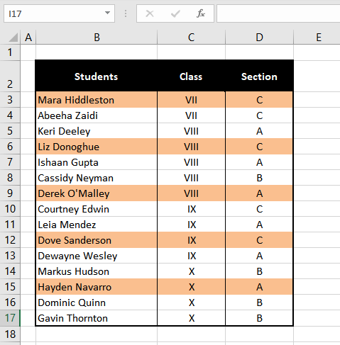
Also, depending on the row where your dataset begins, play around with the remainder in the formula to set where you want the highlighting to begin in the table. E.g. Since our data selection began from row 3, if we were to put 1 as the remainder in the formula, the highlighting would have started from row 3 instead of row 4, with every alternate cell highlighted because of '2' as the divisor.

Do note that if you are to sort and filter the data after highlighting the rows, the data will group differently; the highlighted rows will remain highlighted and group together for the applied sorting and filtering.

If you want to sort and filter data without changing the format as alternately highlighted rows (and exactly which rows are highlighted is not a problem as long as alternate rows are highlighted), then you're better off using table styles which brings us to our next segment.

Method #3 – Using Table Styles

For retaining the format of alternately highlighted rows where the highlighting remains unchanged despite sorting, filtering or changes in the dataset (addition or deletion), learn how to use table styles to format your dataset even if it has no formatting from the get-go. Follow the steps below:

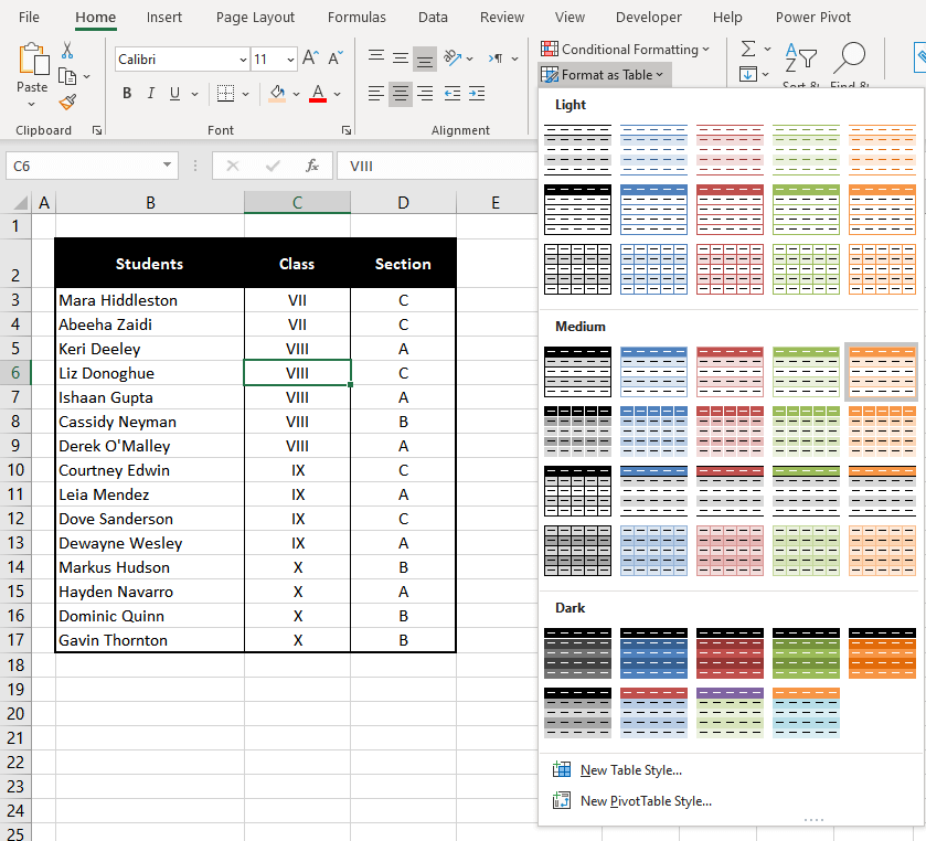
• Select any cell in the dataset. From the Home tab, in the Styles section, click the Format as Table In the drop-down menu, select any table style with banded rows to exhibit the effect of alternately highlighted rows.

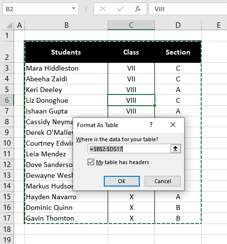
• Once you've selected a style, a Create Table window will pop up with Excel's guess about the range of your dataset. The guess is also depicted by a marching ants border around the dataset on the sheet. Adjust the range here if needed. Leave the My table has headers checkbox checked if your data contains headers. Click OK.

• According to the style selected, the rows in the table should be highlighted alternately.

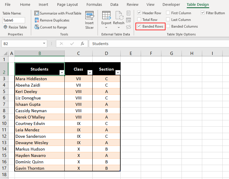
This method not only highlights every other row but also makes a regular dataset a dynamic Excel table which has several helpful features.  If you still don't see alternate rows highlighted, please ensure that the Banded Rows checkbox in the Table Style Options group is checked.

Recommended Reading: How To Add Total Row In Excel Tables

Method #4 – Using VBA

While the above methods are simple and far less daunting, there also stands another option that is VBA. VBA is Visual Basic for Applications where you can use codes to get tasks done in Excel. We'll use VBA for highlighting alternate rows and for what it's worth, here are the steps:

• Select the range to be highlighted and press Alt + F11 to launch the VBA window.

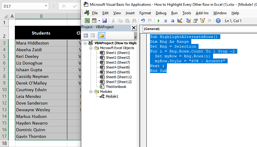
• Click the Insert tab, then click the Module. In the module window, paste the following code:

Sub HighlightAlternateRows()
Dim Rng As Range
Set Rng = Selection
For i = Rng.Rows.Count To 1 Step -2
 Set myRow = Rng.Rows(i)
 myRow.Style = "60% - Accent6"
Next i
End Sub

• Execute the code using F5 key and every alternate row in your selected range gets the new shade as expected.

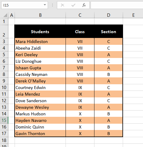
Now, how about some insight on the code.

The above code takes the range selected on the worksheet and using a For Loop iterates over the range. The iterations happen to start from the last row of the range and the step increment value is set to -2. This means instead of iterating over the rows one by one we iterate over every other row from the selected range.

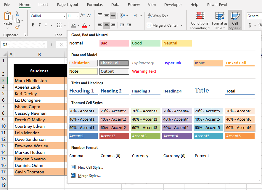
While performing the iteration over the rows, we are setting up the row style as 60% – Accent6 and then proceed on to the next iteration.

You can pick any style (like "Accent1", "Accent2", "Accent3" etc.) from the Styles section in the Home tab to add to the code.

So that was all about highlighting every other row in Excel. What was the highlight for you? Remember you can also highlight columns in similar ways. While you're learning (and highlighting), we're working on placing another brick in the Excel wall for you. Let's see if you can cement it in your minds.