The need for locking cells comes with the ease of editing in Excel. Think of a calculation that has multiple columns referenced within the formula (e.g. net salary using taxes, allowances, and bonus calculations). If accidentally one value is changed, it affects the whole string of calculations and consequently the final amount (not to mention employee morale).
Such things can easily make your spreadsheets a scary thing. However, thankfully we have the option of locking the cells containing formulas to avoid intentional and unintentional tampering and editing; that’s what we will address today.
Locked cells cannot be edited, but it does not restrict us from seeing the formulas in the Formula Bar. While this isn't a problem in most cases, but if you don't want the formulas to be visible, you need to make them hidden. This tutorial will take you through locking formula cells and hiding formulas in Excel.
Notes on Cell Locking and Hiding
This may come as a surprise but all cells are locked by default in Excel. The locked cells however are only truly locked from editing once the worksheet is protected.
Hidden cells also need sheet protection to hide the contents of the cells. This means that both cell locking and hiding need sheet protection to work.
To lock certain cells on a worksheet, all cells must be unlocked first. Then the specific cells can be selected and locked. Next, the sheet has to be protected to lock the cells from being changed.
Lock Formula Cells In Excel
Locking formula cells means that we will be locking some chosen cells. For that, we need to change the default setting of all the cells in the sheet (which is locked) to unlocked. Then we will select the formula cells and lock them. After locking the cells, the worksheet needs to be protected to lock the cells from being edited.
There is a nifty trick to automatically select all the formula cells in a sheet instead of selecting them manually. That nifty trick is to use Go To Special. We will use this feature to select the formula cells in the sheet to lock them.
Below are the steps to unlock all the cells, lock the formula cells and protect the worksheet. Let’s break them down, one by one.
Step 1 – Unlock all the Cells in the Worksheet
- Select all the cells in the worksheet (Ctrl + A).
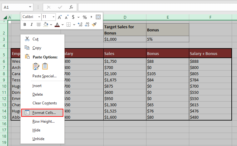
- Launch the Format Cells dialog box by right-clicking any cell and selecting Format Cells from the right-click context menu (or using the keyboard shortcut Ctrl + 1).
- In the dialog box, go to the Protection The Locked checkbox will be ticked. Uncheck the Locked checkbox.
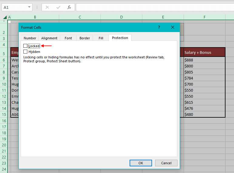
- Click OK.
Now all the cells on the sheet are unlocked. This will not have any visual impact on the sheet unless the data contains formulas. In that case, you will see a green arrow in the top left corner of all formula cells. Selecting any of these cells will show the Trace Error button which will report exposed formulas due to unlocked cells.
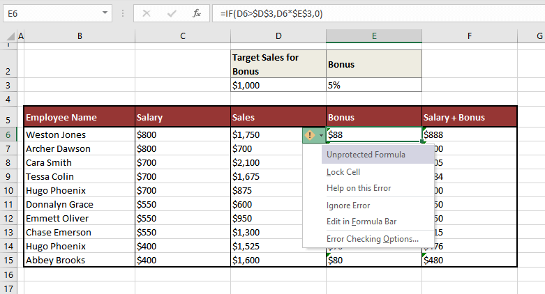
Don't worry locking these cells will fix this error and that is our next step.
Step 2 – Lock the Cells in the Worksheet Containing the Formulas
Now we will lock only the formula cells in the worksheet so that after the sheet is protected, only the formula cells cannot be changed. Instead of selecting the formula cells manually, we will use the Go To Special feature. Below are the steps to lock the formula cells in the worksheet with Go To Special:
- Select all the cells in the worksheet (Ctrl + A).
- In the Home tab, from the Editing section, click on the Find & Select From the drop-down list, select Go To Special to open the Go To Special dialog box.
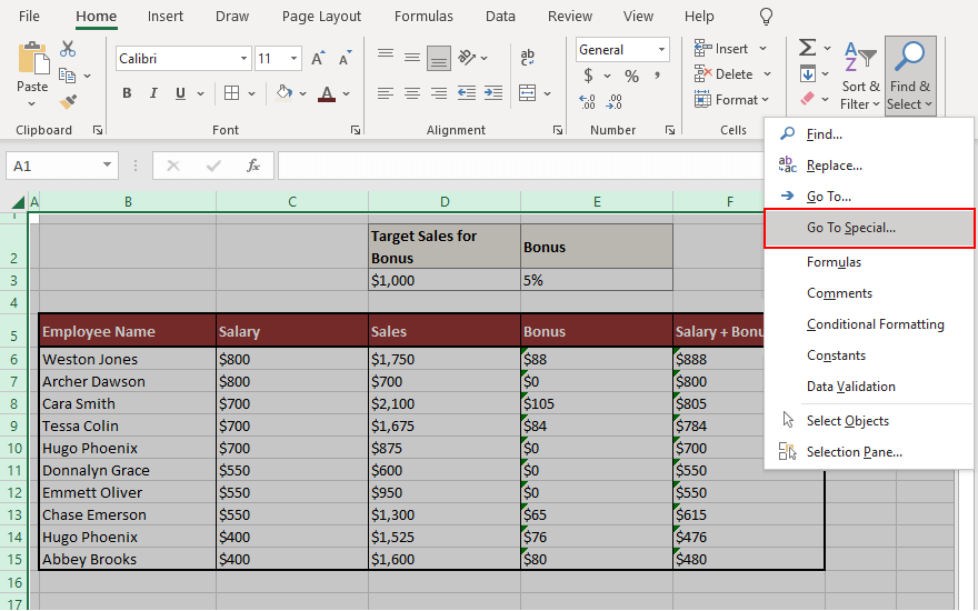
- Select the Formulas radio button and make sure all the checkboxes under Formulas are checked. Then click OK.
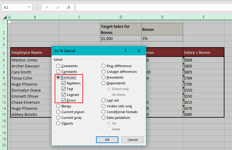
As you can see below, all cells containing formulas on the worksheet will be selected.
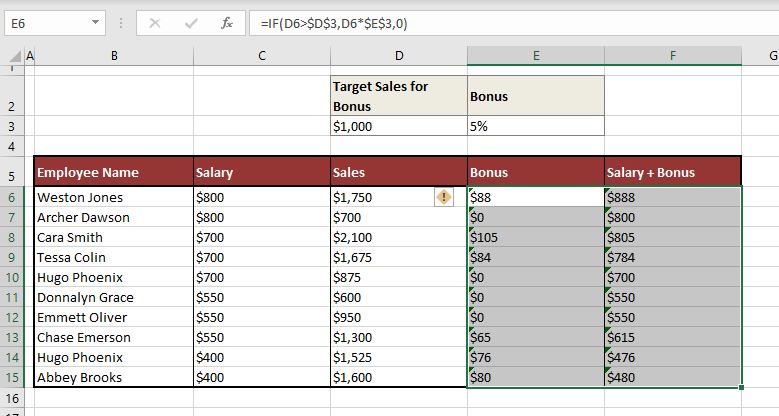
The next step is to lock the selected formula cells.
- Launch the Format Cells dialog box by clicking on the dialog launcher (small arrow on the bottom right) in the Alignment section (or use the keyboard shortcut Ctrl + 1).
- In the Protection tab, check the Locked Then click OK.
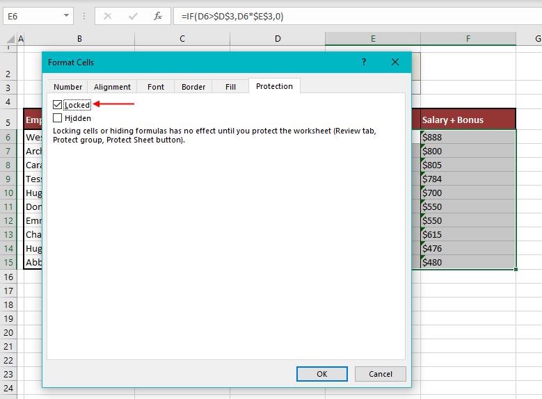
Now that the formula cells are locked, the formula errors have disappeared.
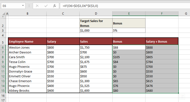
To completely restrict the editing of locked cells, the worksheet needs to be protected, which is the next step.
Step 3 – Protect the Worksheet
To activate the properties of a locked cell, you have to protect the worksheet and the simple steps for doing that are as follows:
- Go to the Review From the Protect section, select the Protect Sheet command button.
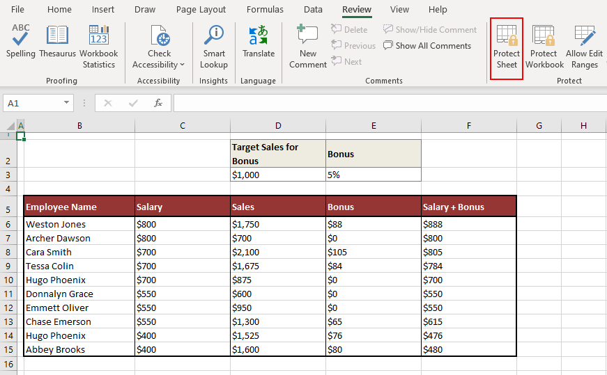
- Confirm that the Protect worksheet and contents of locked cells checkbox is checked.
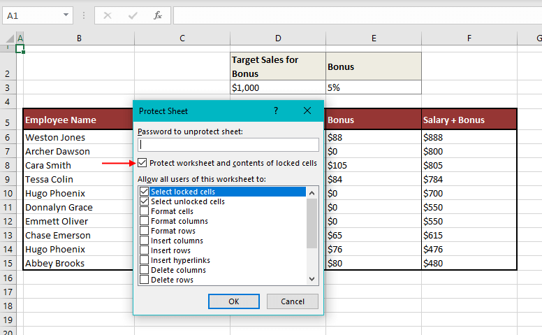
- In this Protect Sheet dialog window, you have the option of adding a password to unprotect the sheet. It can be helpful to keep a password to allow some users to edit the locked cells by sharing the password with them.
- Other controls of the worksheet are in Allow all users of this worksheet to: field. We are going with the default settings (top 2 checkboxes checked).
- After making the changes as you like, click OK.
Following these steps have protected the worksheet and locked the formula cells, disallowing any editing. Any cell other than the formula cells can be edited. Should you try to edit a cell containing a formula, a prompt will pop up notifying that the cell belongs to a protected sheet.
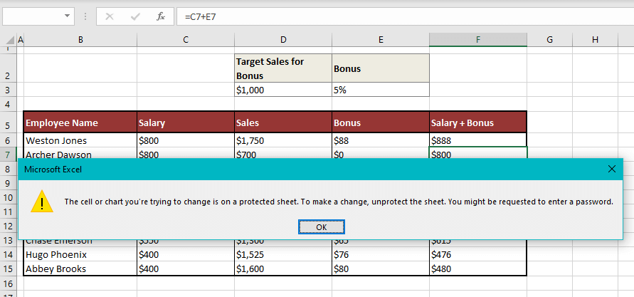
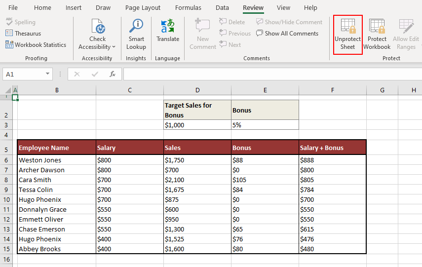
If a password had been set up in the Protect Sheet window, the user will be asked to enter the password while unprotecting the sheet from the Unprotect Sheet command button in the Review tab. With no password, the sheet can be unprotected by clicking the Unprotect Sheet command button straight away.
Recommended Reading: All About Locking & Protecting Worksheets
Hide Formulas In Excel
By hiding formulas, the formula of the cell will not display in the Formula Bar when the cell is selected. The process of hiding formulas is very similar to that of locking cells (with just an extra setting enabled). Like locked cells, hidden cells also work only once the sheet is protected.
The formula cells have to be selected to be hidden. We will use the Go To Special feature to select the formula cells to hide them. Here are the steps to select and hide the formula cells and to protect the sheet:
- Select all the cells in the worksheet (Ctrl + A).
- In the Home tab, from the Editing section, click on the Find & Select From the drop-down list, select Go To Special to open the Go To Special dialog box.

- Select the Formulas radio button and make sure all the checkboxes under Formulas are checked. Then click OK.

- All cells containing formulas on the worksheet will be selected like so:

The next step is to hide the selected formula cells.
- Launch the Format Cells dialog box by clicking on the dialog launcher (small arrow on the bottom right) in the Alignment section (or use the keyboard shortcut Ctrl + 1).
- In the Protection tab, check the Hidden Then click OK.
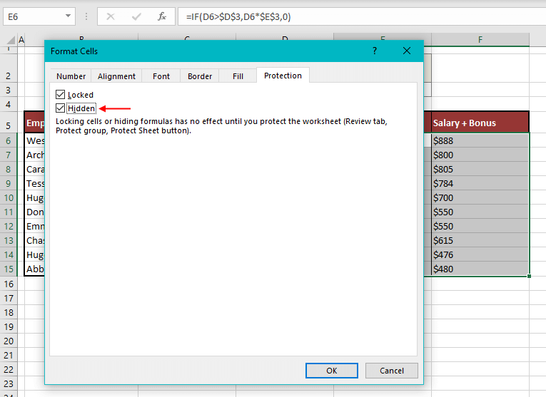
This has no visual impact on the sheet yet as the hidden properties only work once the sheet is protected. If you select any of the hidden cells right now, you can still see the formula in the formula bar. Let’s move on to protecting the sheet:
- Go to the Review From the Protect section, select the Protect Sheet command button.

- Confirm that the Protect worksheet and contents of locked cells checkbox is checked.

- In this Protect Sheet dialog window, you have the option of adding a password to unprotect the sheet. It can be helpful to keep a password to allow some users to edit the locked cells or view the formulas by sharing the password with them.
- Other controls of the worksheet are in the Allow all users of this worksheet to: field. We are going with the default settings (top 2 checkboxes checked).
- After making the changes as you like, click OK.
Following these steps have protected the worksheet and hidden the formula cells. If you select any cell containing a formula now, you can see that the Formula Bar will not display its formula.
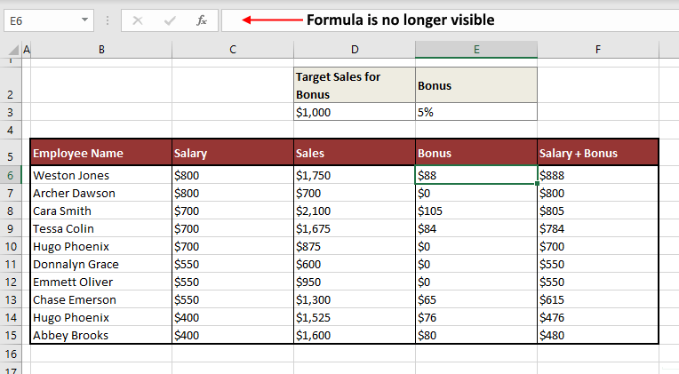
If you had set up a password in the Protect Sheet window, the user will be asked to enter the password while unprotecting the sheet from the Unprotect Sheet command button in the Review tab. With no password, the sheet can be unprotected by clicking the Unprotect Sheet command button.

Recommended Reading – Excel Shows Formula Instead of Result (How to Fix)
VBA to Lock and Hide Formulas In Excel
You can ditch all the steps above and select, lock and hide formulas and protect the worksheet using VBA. All you have to do is access the VBA editor, feed in the right code, run the command and that’s job done!
VBA (Visual Basic for Applications) is a programming tool for MS Office applications. We can use codes in VBA to get various tasks done in Excel, especially if they are laborious or repetitive.
Below we will show you how to use VBA to lock and hide formulas and protect the sheet, all using one code. The steps are:
- Press Alt + F11 to run the VBA editor. If you don’t have the Developer tab, you can add it by customizing the ribbon and then access the VBA editor using the Visual Basic button.
- Click on the Insert tab and select Module from the list.
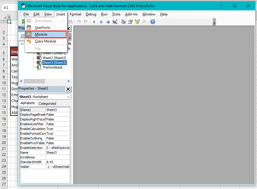
- In the opened module window, copy and paste the following code:
Sub LockAndHideAllCellsWithFormulas()
With ActiveSheet
.Unprotect
.Cells.Locked = False
.Cells.SpecialCells(xlCellTypeFormulas).Locked = True
.Cells.SpecialCells(xlCellTypeFormulas).FormulaHidden = True
.Protect AllowDeletingRows:=True
End With
End Sub
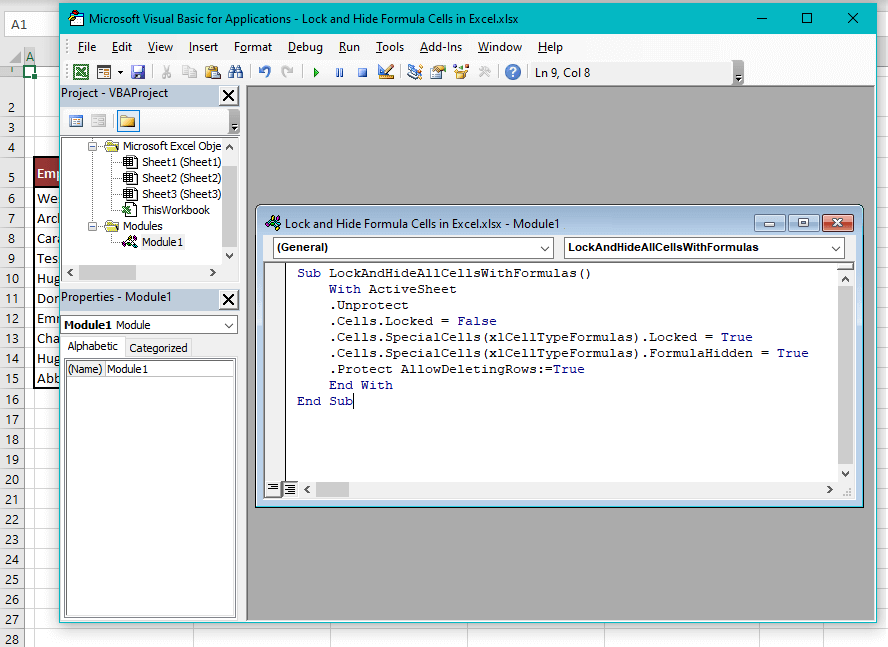
- Close the module window and the VBA editor.
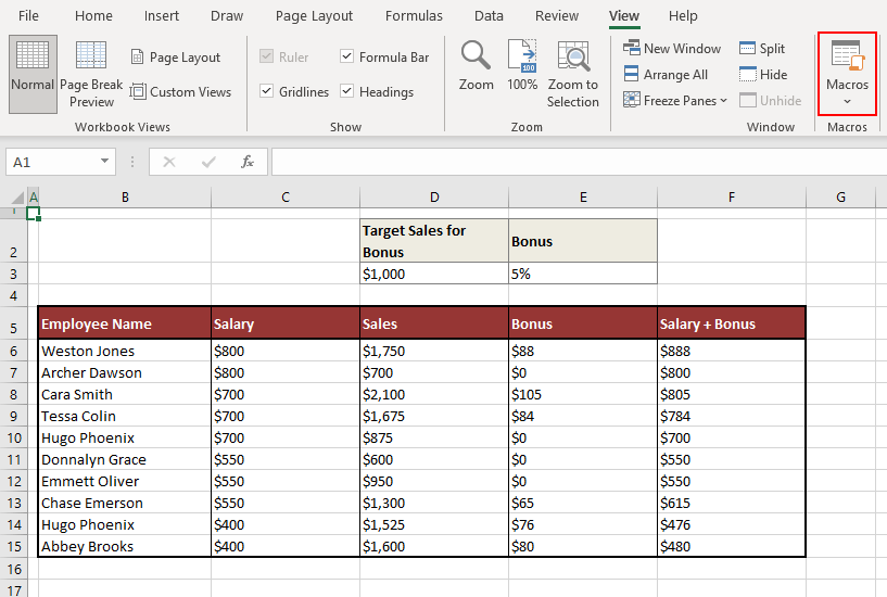
- Go to the View tab and select the Macros command button.
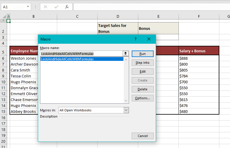
- Select the relevant macro and then select Run.
Using the above-mentioned code, we have locked and hidden the formula cells and protected the sheet. If you try editing a formula cell, you will receive a prompt, disabling you from editing. That confirms the formula cells are locked.
Selecting any formula cell, you can see below that the formula is not visible in the Formula Bar. This confirms the formula cells are hidden.
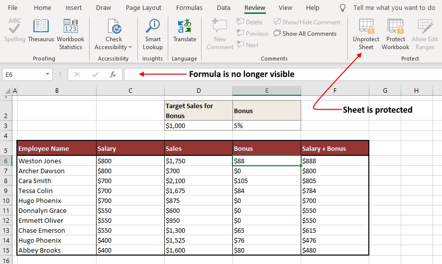
Both the locked and hidden properties are working which means the sheet is protected which is also confirmed from the Review tab.
Now let’s lock that up and stop right here. We hope we gave you the full particulars on protecting the formula cells from all sorts of tweaking. We’ll be back, unlocking and unraveling more Excel mysteries; be ready to keep up!


