How To Insert a Checkmark Symbol (✓)  In Excel

A checkmark or a tickmark can be used in Excel and this is the face of it – ✓

Why do you need a checkmark in Excel? Most commonly, a checkmark says "Done". A more representable way of having "Done" and "Not Done" or "Yes" and "No" on the worksheets can be ticks and crosses. If that reminds you so much of a teacher's red ink on your work, let's call them checkmarks and crossmarks.

There are many ways of inserting checkmarks in Excel. This tutorial will guide you through several methods involving shortcuts, formulas, VBA, and different settings and features which will make adding checkmarks a breeze. There are plenty of options so let's get started! But first, let's clear up that we are talking about checkmarks today, not checkboxes. Read ahead.

Difference Between a Checkmark and Checkbox

A checkbox is an interactive graphical widget that allows the user to check it with a checkmark or leave it unchecked (blank). The graphical part of the checkbox clarifies that it isn't text and therefore not part of cell text and not part of a cell. Therefore, it sits above the cell as an object and is unaffected by the contents of the cell or movement/deletion of the cell. That also means the checkbox can be freely moved anywhere on the sheet.

A checkmark is a text symbol and therefore is part of a cell, like any text. Being the content or part of the content of the cell, a checkmark is affected by the movement of the cell (a copy-pasted cell will also copy-paste the checkmark in it. And a deleted or moved cell will delete or move the checkmark with it). A cross mark can also be used in the same way as a checkmark. This also differs from a checkbox which can only be either checked or unchecked.

If you are looking to add checkboxes instead of checkmarks, check out our detailed guide on checkboxes here – Everything You Need to Know About Excel Checkboxes

Now that we've established that this guide is about checkmarks, let's explore many ways of adding them to our sheets.

Method #1 – Insert Checkmark Using CHAR Function

The CHAR function returns a character against a specific code entered in the function. In this way, we can use the CHAR function to return a checkmark in Excel. A requirement is that the font of the cell must be set to Wingdings as it is a symbol font. Hence, we can have a checkmark as a text symbol using Wingdings and the CHAR function.

With the Wingdings font, here are the codes that we need to feed in the CHAR function to arrive at a checkmark or a cross mark:

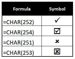
The first step would be to change the font of the cells where the check and cross marks will be entered to Wingdings.

The code for a checkmark is 252. So, we will feed 252 into the CHAR function like so:

We can manually use the CHAR function with the relevant codes to add check and cross marks in the data below:

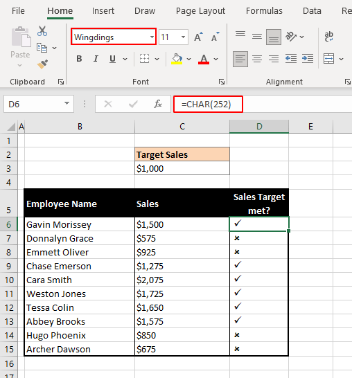
But with Excel around, it seems a little sad that we should do so much work manually. Thus, we can add the IF function into the works so a check or cross mark can be conditionally returned. This is the formula we will use:

The function reads like this: If C6 is greater than C3, return CHAR(252). If not, then return CHAR(251). This means that if the sales is greater than the target sales, return a checkmark. If not, then return a cross mark. The target sales figure is locked in the $ signs to keep it as a constant in the formula as the formula is dragged.

Here we have the results of this formula:

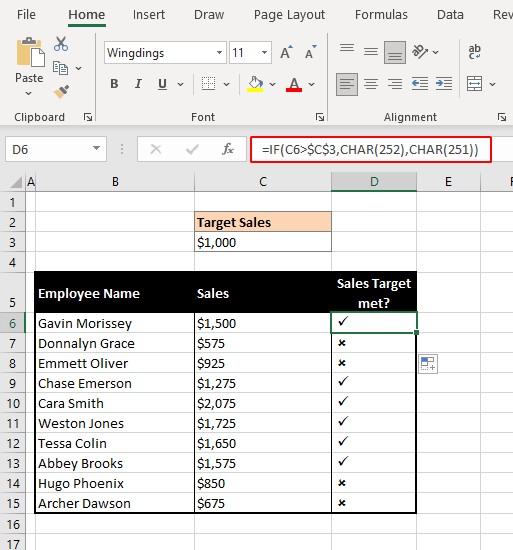
You can also use the boxed check and cross marks, whichever is the preference.

Easy-peasy, isn't it?

But every time you may not have data where you need to conditionally enter checks and crosses such as to-do lists. For punching them in, there are other options mentioned in the following sections.

Method #2 – Insert Checkmark Using Copy Paste Checkmark

And of course, the simple copy-paste. No frills, no strings, copy from here and paste to the cell where you want the checkmark: ✓

• Copy the checkmark above.
• Select the cell where you want the checkmark and go into cell edit mode (by pressing F2 or using the formula bar).
• Paste the checkmark in the cell or formula bar.

You can also use the other Paste Options instead of going into cell edit mode.

And you should have your checkmark ready!

Method #3 – Insert Checkmark Using Keyboard Shortcut

To quickly and easily add a checkmark, you can make use of keyboard shortcuts. Before you do, change the font of the designated cell(s) to Wingdings 2 or Webdings font as per the below table.

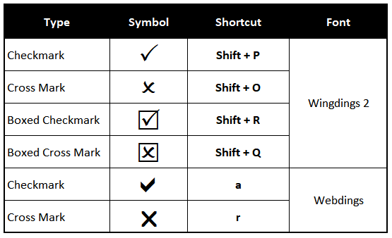
Using the above keyboard shortcuts, we can get checkmarks and cross marks as text symbols.

Method #4 – Insert Checkmark Using AutoCorrect

AutoCorrect needs no introduction but let's remind ourselves of its basic properties to see how we can use it for inserting checkmarks. Autocorrection is automatic text replacement for spelling or typing errors. We can tinker with the AutoCorrect settings to replace a keyword with a checkmark or even a cross mark. Sounds handy? Let's get our hands on this:

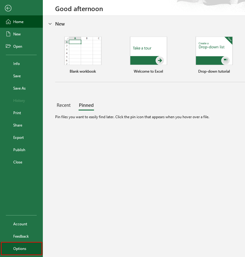
• Click on the File tab and go to Excel Options.

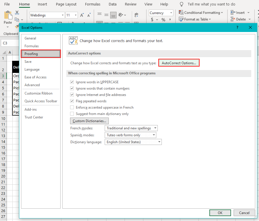
• Select Proofing from the side panel. Now select AutoCorrect Options to open the AutoCorrect dialog window.

• In the Replace: field, add a keyword of your choice that you will have to type in the cell to insert a checkmark. We have set "CHMARK" for a checkmark.
• In the With: field add the checkmark symbol ✓ (you can copy and paste this)

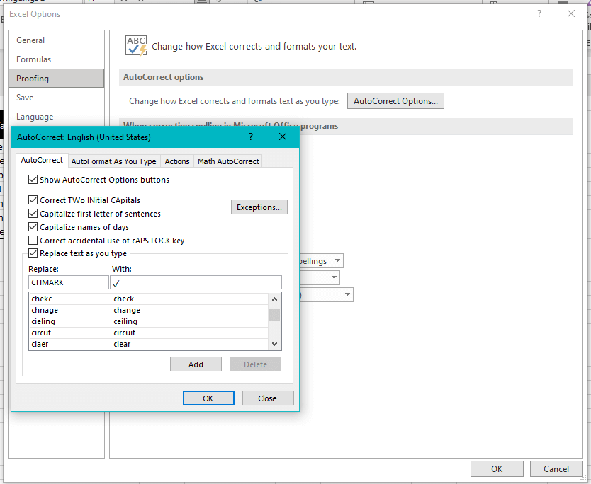
• Click Add.

Now to set up the keyword for a cross mark:

• In the Replace: field, add a keyword of your choice that you will have to type in the cell to insert a cross mark. We have set "CRMARK" for a cross mark.
• In the With: field add the cross mark symbol ☓ (you can copy and paste this)

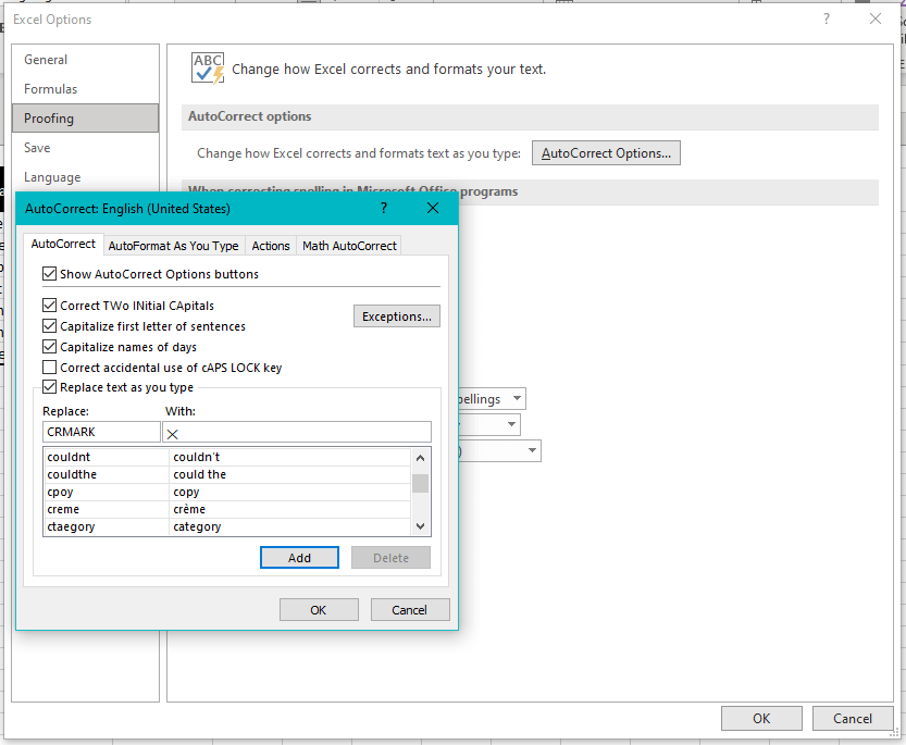
• Click Add. Then click OK on both the dialog windows to initialize the settings.

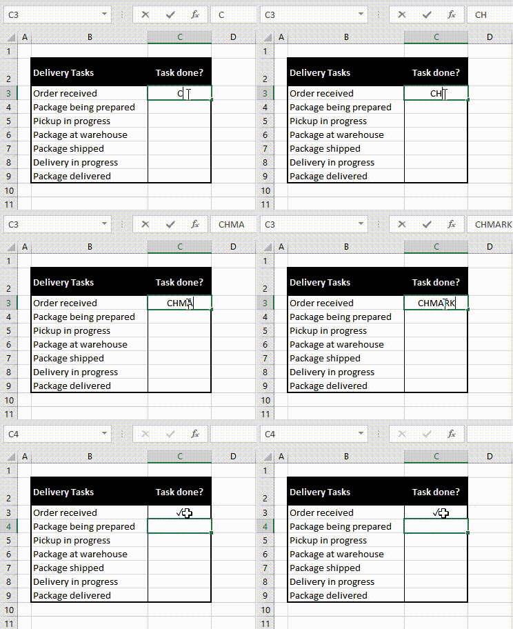
Now select the cells where the checkmarks are required. Type CHMARK in a cell, hit Enter and you will see the checkmarks getting generated.

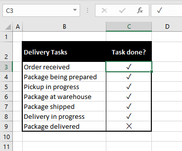
Voila! Checkmark on display! There's the cross mark too.

Notes:

The keyword is case sensitive; you must use the case set for the keyword in the AutoCorrect options.

The AutoCorrect options apply to all the MS Office applications so, the keyword can be used in other applications too.

There are a few other ways to set the replacement text for a checkmark and depending on the method; you may use the keyword with other text in a cell to get a checkmark; keyword separated from other text by a space character.

Method #5 – Insert Checkmark Using Conditional Formatting

According to the value of a cell, we can conditionally format the cell to return a checkmark. Let’s say we have a sales target and want a checkmark or a cross mark against our sales data indicating target achieved or not. With a few settings, this is doable so let’s see the steps.

• Copy and paste the sales column to the next column and select all the values in the pasted column.

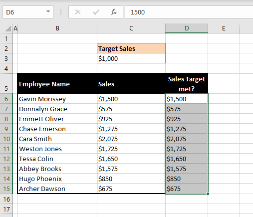
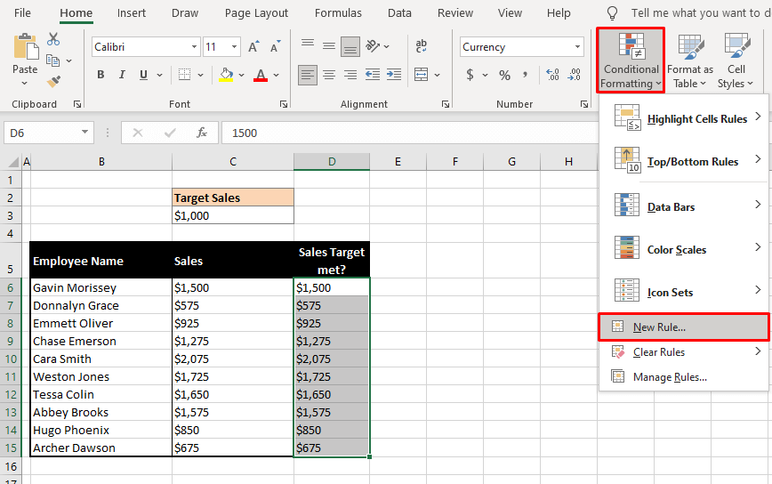
• In the Home tab, in the Styles section, select Conditional Formatting.
• Select New Rule… from the drop-down list. This will open the New Formatting Rule dialog window.

• From Format Style: select Icon Sets from the list.

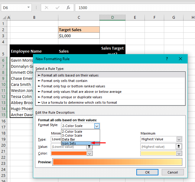
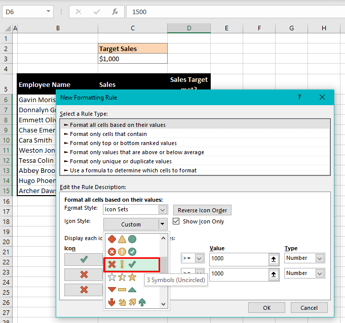
• From Icon Style: select the style with the cross, exclamation, and checkmark.

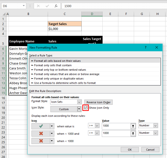
• Check the Show Icon Only

• In the Type section, change both the options to Number.

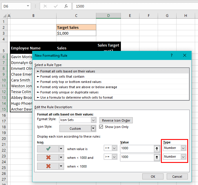
• In the Value section, enter 1000 in both fields.

This is the target number against which you want to measure up the data on the worksheet.

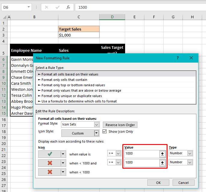
• In the Icon section, set the icons to checkmark, cross mark, cross mark.

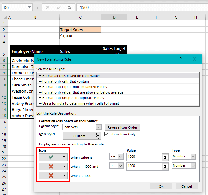
• Click OK.

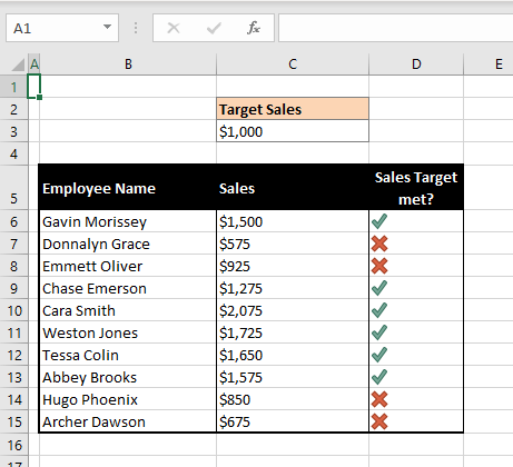
And that’s how we use conditional formatting to format values meeting our target into checkmarks and values below target into cross marks. There are other ways you can use Conditional Formatting such as using a formula involving the CHAR function to return a checkmark.

For a simpler to-do list where you need to just add a checkmark or a cross mark, you can feed 1 and 0 instead of the sales target. Here’s how:

• Select the cells where you want to insert the check and cross marks.
• Go to Home tab > Conditional Formatting button > New Rule…

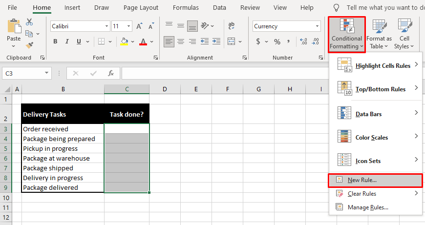
• From Format Style: select Icon Sets from the list.
  • From Icon Style: select the style with the cross, exclamation, and checkmark.
  • Check the Show Icon Only checkbox.
  • In the Type section, change both the options to Number.
  • In the Value section, enter 1 in the first field.
  • In the Icon section, set the icons to checkmark, cross mark, cross mark.

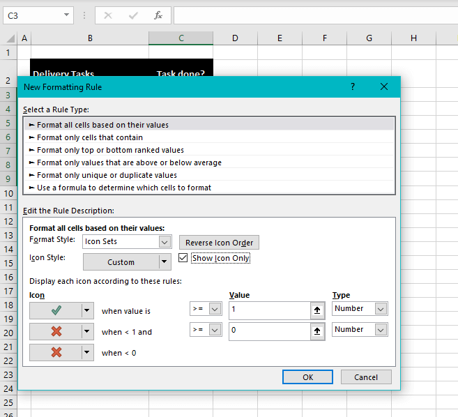
• Click OK.

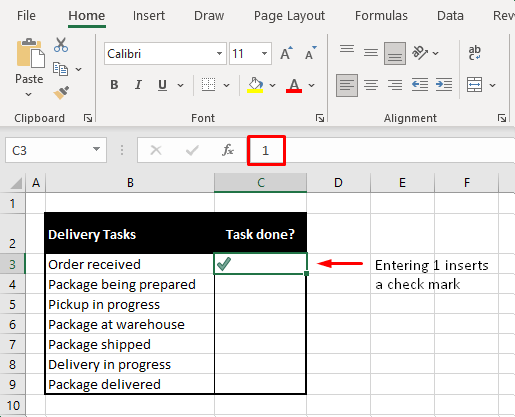
Back to the cells, enter 1 where you want the checkmark.

Enter 0 where you want the cross mark.

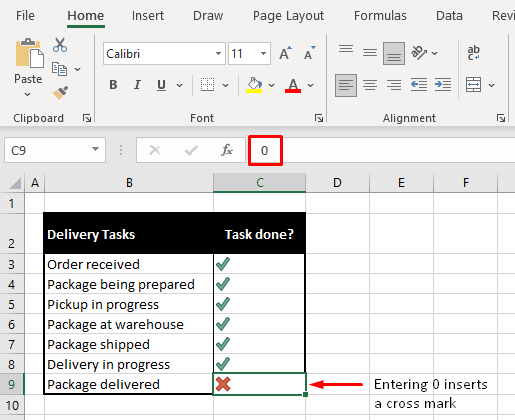
Checks and crosses dealt with!

Method #6 – Insert Checkmark Using Macro (VBA)

For tasks that you need to do in volume or need done regularly, VBA can quickly become your BFF. VBA, Visual Basic for Applications is a Microsoft programming tool. Here, we can program Excel using codes in VBA for recurring or regular tasks. Now we will show you how to use a code for returning checkmarks:

• Press Alt + F11 to launch the VBA editor.

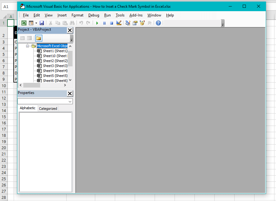
• From the Insert tab, select Module from the drop-down list. This will pop open the Module window.

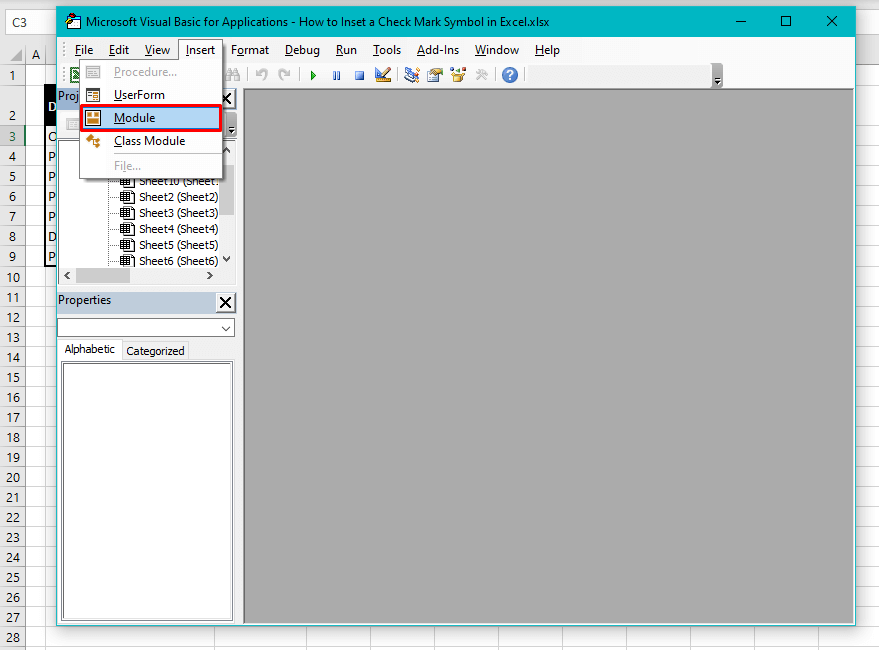
• Copy the following code and paste it into the field in the Module window:

Sub addCheckMark()
Dim rng As Range
For Each rng In Selection
 With rng
 .Font.Name = "Wingdings"
 .Value = "ü"
End With
Next rng
End Sub

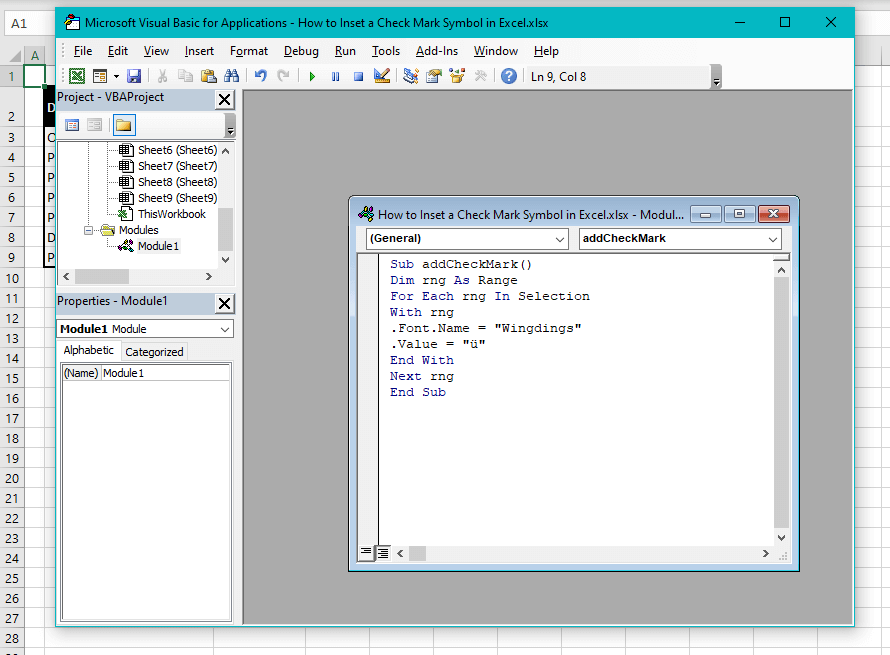
• Add another Module by selecting Module from the Insert

This one is for adding a cross mark.

• Add the same code to the Module field but change CheckMark into CrossMark in the first line and change ü to û in the 6^th Or you can copy and paste the following code:

Sub addCrossMark()
Dim rng As Range
For Each rng In Selection
 With rng
 .Font.Name = "Wingdings"
 .Value = "û"
End With
Next rng
End Sub

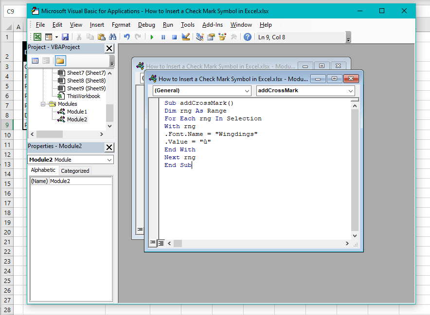
• Close the Module windows and the VBA editor.

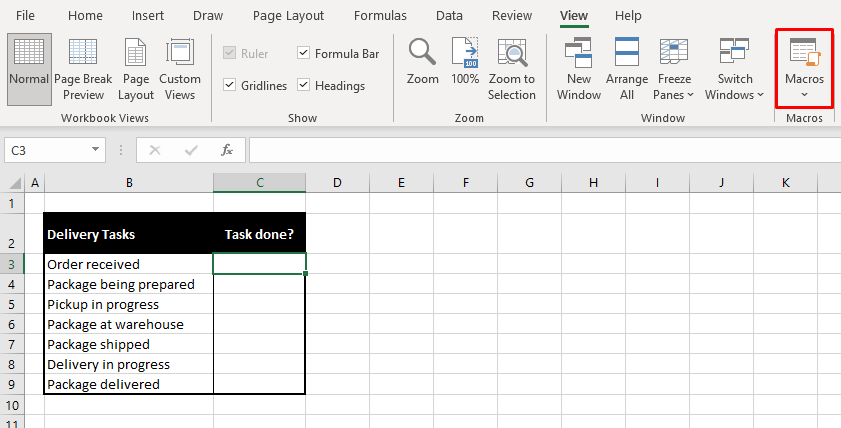
• Select the cells where you want to place the checkmark.
• Go to the View, Select the Macros command button to open the Macro dialog window.

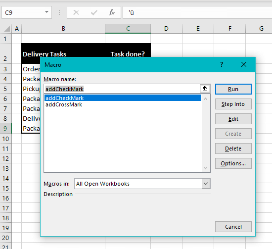
• Select the checkmark macro and hit the Run

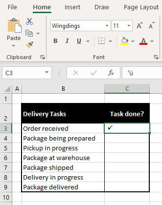
And the checkmark will take no time in presenting itself:

Or a cross mark for that matter:

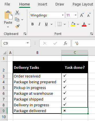
The ease of using Macro is that there is no prerequisite to change the font of the cells because the code loops through the selected cells, changing the font to Wingdings and inserting the value ü in the cells. ü is the value in the Wingdings font for a checkmark and û for a cross mark.

Method #7 – Create a Dropdown to Insert Checkmark

Another option is to create a drop-down list from which you can select the checkmark for every cell individually. This option utilizes the Data Validation feature and here are the steps:

• Select the cells where you want to insert the checkmarks.
• Go to the Data tab and select the Data Validation command button to open the Data Validation dialog window.

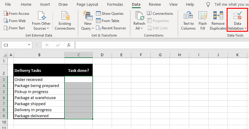
• In the dialog window, from the Allow: options, select List.
  • In the Source: field, add the checkmark symbol: ✓ (copy from here)
  • If you want to add a cross mark too, add it to the Source: field with the checkmark, separated by a comma. ☓ (copy from here)

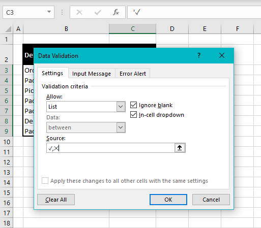
• Click OK.

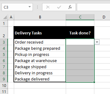
These steps will set up individual drop-downs for each cell selected in the first step.

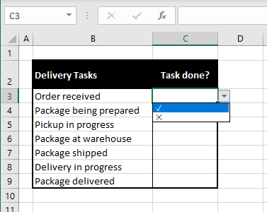
• Click on the little arrow to access the drop-down and you will see your added checkmark and cross mark. Select and done!

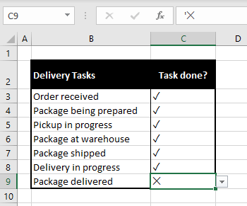
You can keep adding check and cross marks for the rest of the cells.

Formatting Checkmark in Excel

A checkmark is a text symbol (unless it has been entered as an image) and like any text, it can be formatted. Meaning, you can change the color, size, etc like any text.

Let’s copy column C in the example below to column D and format the check and cross marks. Below, we have emboldened the check and cross marks.

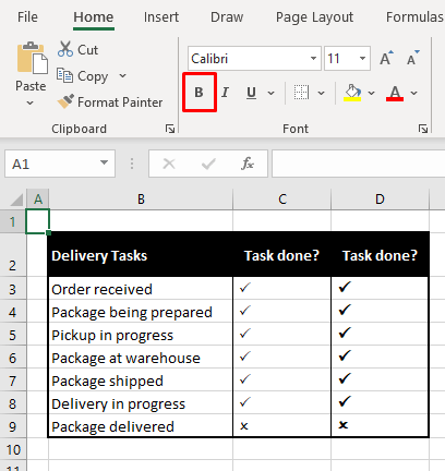
Next, we’ve changed the font size.

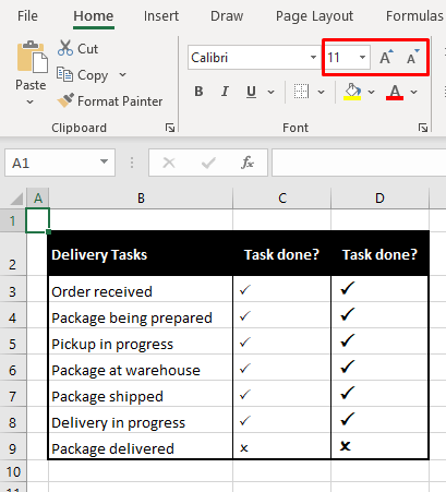
And then we’ve changed the font color.

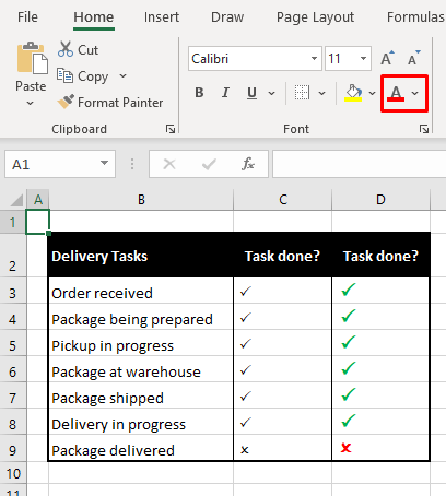
All text formatting can be applied to checkmarks and cross marks when they are inserted as text symbols.

How to Count Checkmarks in Excel

For counting the number of checkmarks on our sheet, we can use the COUNTIF function with the CHAR function. Let’s briefly find out what the two functions are and why we need them together.

The COUNTIF function counts (no kidding) the number of cells within a range meeting the given condition. As mentioned earlier, the CHAR function returns a character against a specific code entered in the function.

We will use CHAR(252) in the formula which is the CHAR code using the Wingdings font for a checkmark. We will use this code in the COUNTIF function to count the number of checkmarks.

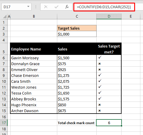
Let’s refer to our example:

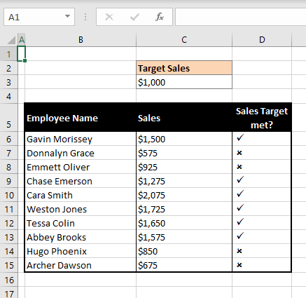
Say we want to count how many employees met the sales target which means we want to count the checkmarks. Here’s the formula we will use to count the checkmarks:

The COUNTIF function counts the number of cells containing CHAR(252) (i.e. checkmarks) in the range D6:D15. The result is 6 which means there are 6 checkmarks in cells D6:D15 and hence, 6 employees who met the sales target.

And with that, we mark the end of this tutorial. We’re certain, checkmarks can make their way into your worksheets from one of the several ways above. Learned ways to add tick marks? Check. Learned fancy things to do with tick marks? Check. We’re going good! But of course, we’ll be back with more goods from the Excel truck and can’t wait to hand them out!