How to Create, Use, Edit and Delete Named Ranges in Excel

Names are one convenient identity. Imagine how we'd be addressed if we didn't have names? Excel tries to make our lives easier by providing us with a similar convenience.

What are Named Ranges

In Excel, a cell or a range of cells can be named to make their usage easier. It would be simpler to use a named range directly in a formula or select said range.

You can name:

• a Range of cells,
• a Formula,
• a Constant or
• a Table

Benefits of Creating Named Ranges in Excel

• The prime advantage of named ranges is the ease they provide. You don't have to keep glancing at certain cells or tables to pick up values or cell references and can use a named range instead.
• Using a named range will save typos that may otherwise occur while typing values or formulas since entering named ranges is a clickable option.
• They are of great help to use in formulas as the named range appears upon typing the first letter of the name.
• Named ranges make formulas movable and they can be used from sheet to sheet and workbook to workbook.
• A dynamic named range can automatically account for expanding and contracting data (when values are added or deleted from a dataset) without having to change the formula or recalculate.
• A named range can be used for data validation (creating drop-down menus) without much hassle.
• Hyperlinks can quickly be created from existing named ranges.
• Named ranges make navigation and directing very easy. You can click on a named range in the Name Box and arrive at the named range.
• For all the above benefits that named ranges deliver, they are very simple and quick to create.

Rules for naming Named Ranges

There are several pointers not to trespass while creating named ranges:

• A name should have less than 255 characters.
• A name should not have space and punctuation characters (exceptions mentioned as follows).
• A name's first character has to be a letter, an underscore ( _ ), or a backslash ( \ ).
• A name may contain a question mark but never as a first character.
• A name is not case-sensitive. (sale, Sale, and SALE are treated as one name).
• A name must not resemble a cell reference (e.g., A1, A$1).
• A name may be a single letter name but must not be r, R, c, or C as "R" and "C" signify row and column selection shortcuts.

How to Create Named Ranges in Excel

There are two methods to create named ranges in excel. We will see both these methods in this section.

Let's say we have the data as shown below and we want to create two named ranges – one for the History marks and the second one for the Geography marks.

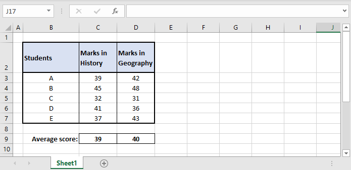
We will create these two named ranges using two different methods to help you get a hang of both methods.

Method 1 – Creating Named Ranges from the Name Box

The how-to here is pretty simple. Select the range, enter the desired name in the "name box" and press Enter. Done! Really! We can show you how easy this is with a visual.

Here's how it's done:

• For naming the History marks range, we will select the History marks i.e., range C3:C7.

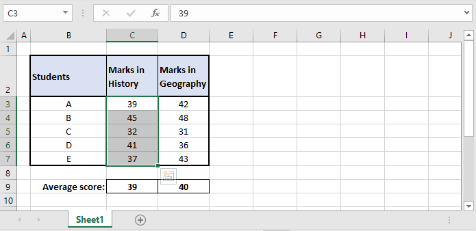
• Click on the name box.
• Enter the desired name ("History" in this case).

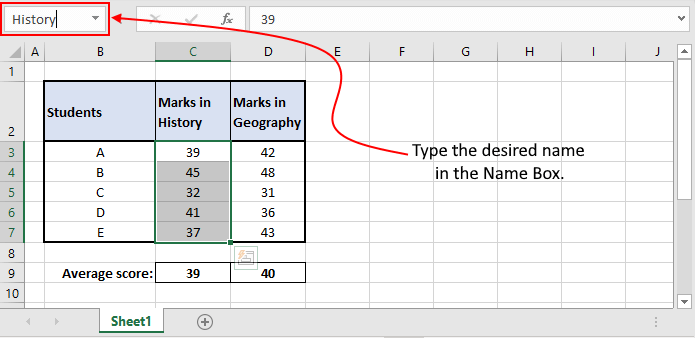
• Press the Enter key.

Method 2 – Creating Named Ranges from the 'Define Name' Option

Names can also be created from the  "Define Name" button, in the formulas tab. To use this method follow the below steps:

• Select the range which you want to name, in our case it will be D3:D7.
• Navigate to the "Formulas Tab" and click the "Define Name" button.

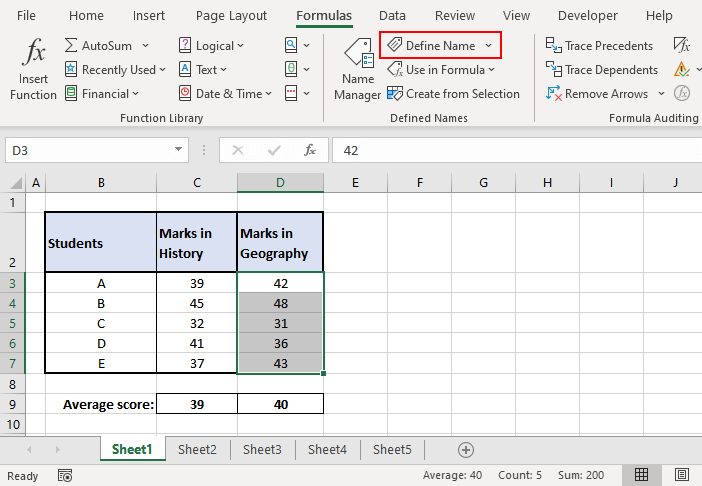
• Now, in the "New Name" window enter the desired name for the named range.

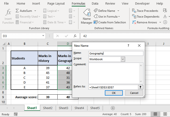
• After entering the desired name click the "OK" button and it is done.

How to Edit Named Ranges in Excel

Suppose you accidentally missed a cell in the range or want to change the name of your named range. This means the named range needs to be edited.

Named ranges can be managed through the "Name Manager" which can be found under the "Formulas" tab > Name Manager or can be accessed through the keyboard shortcut Ctrl + F3.

This is what you will see when you open the Name Manager:

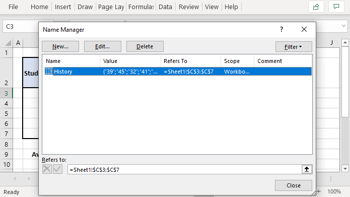
Here, you can see the named ranges in your sheet and their details. Double click the named range you wish to edit or select the named range and click the "Edit…" button.

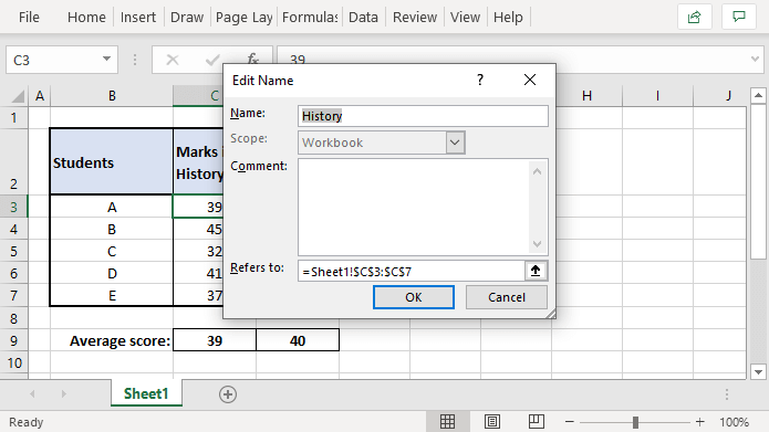
Clicking on the "Edit…" button will open the "Edit Name" window where you can edit the name or the cell range of the named range. When done, click "OK" and then click the "Close" button on the Name Manager.

How to Delete Named Ranges

The Name Manager can also be used to delete named ranges. Click the named range you wish to remove, press the "Delete" button.

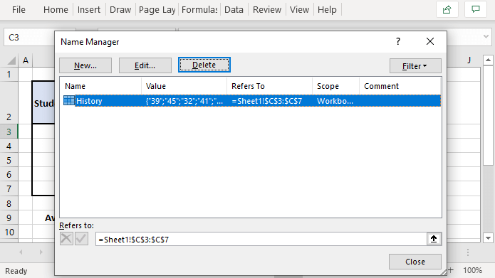
You will get a pop-up confirmation asking whether you want to delete the named range or not. Press "OK" and that will delete your chosen named range.

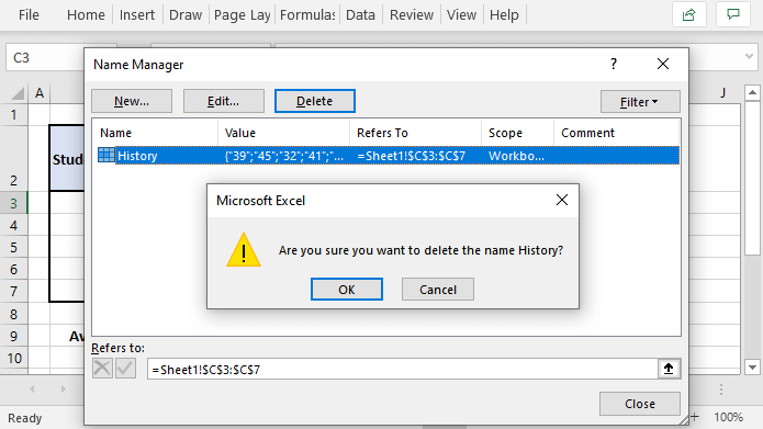
Note that the Name Manager also has a "Filter" button that can be used for filtering the names and only viewing the relevant names at a given time. It can be quite handy when you have a lot of names to deal with.

Recommended Reading: How to Lock and Protect Cells in Excel

How to Create Names from Cell Text

For batch information where the data is in the columnar or row format (i.e., in either columnar form with headings at the top and its relevant data below. Or in rows with headings on the left and its data on the right) there is a quicker way of naming ranges. We can use the "Create from Selection" feature in Excel to give the heading's name to the range. Here is how:

So, we have the dataset containing marks scored by students in various subjects. The layout is in columnar form. We can use the "Create from Selection" feature in this case as –

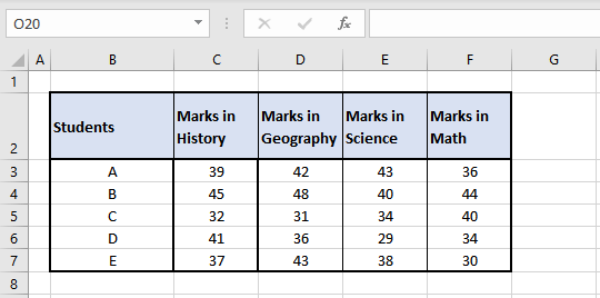
• Select the range and the heading. We will select columns C, D, E, and F to name each range according to its heading.

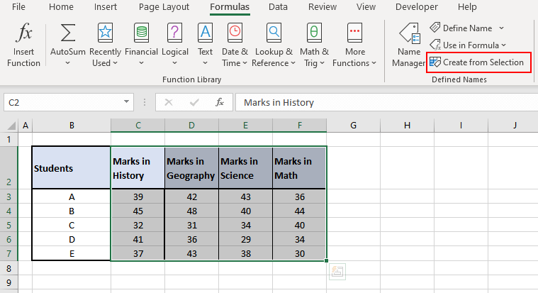
• In the "Formulas" tab, click "Create from Selection" or use the keyboard shortcut Ctrl + Shift + F3. This is what you should see:

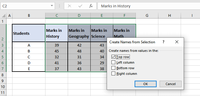
• According to the layout of your dataset, select the row or column where the headings need to be picked from. For our case, we will select the "Top row" option as headings. "Marks in History", "Marks in Geography", "Marks in Science", and "Marks in Math" are in the top row.
• After selecting the appropriate options click "OK".

Doing this has created multiple named ranges for our data. You can see from the drop-down in the Name Box that we have 4 named ranges created according to the headings of each column.

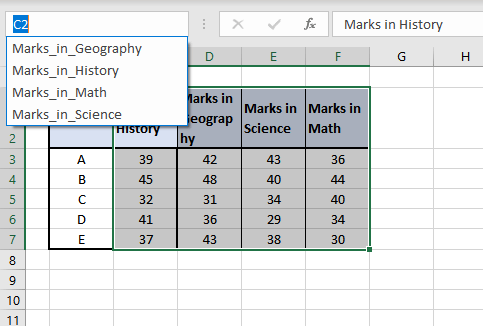
Note that the spaces in headings are replaced with underscores while creating the names.

Named Ranges with Hyperlinks

If you thought named ranges made you bounce around with ease through worksheets, wait for their synergy with hyperlinks. Named ranges make hyperlinking a smoother process as data required for hyperlinking would already be grouped and named. Let's show you how this will work.

For the sake of this example let's assume that we have another named range "Student" in Sheet2 as shown.

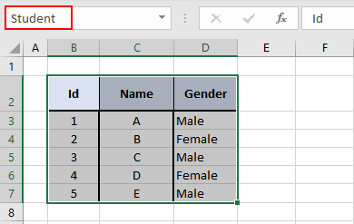
We will hyperlink the Student column from Sheet1 to direct us to the student range in Sheet2.

• Select the Student range in Sheet2 (i.e., B3:B7).

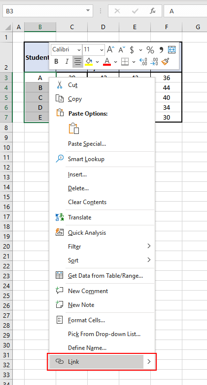
• Right-click the selected area and click on "Link". The "Insert Hyperlink" window is what you should see.

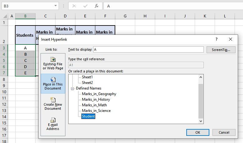
• We will select "Student" from "Defined Names" which we have already defined in Sheet2.
• Click "OK".

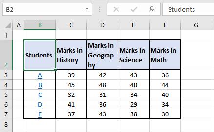
We have hyperlinked the Student Names to Sheet2 using the "Student" named range. Clicking on any of the marks should take us to the "Student" range on Sheet2. Let's check.

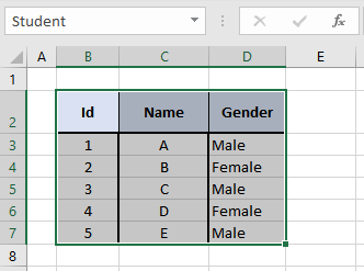
Affirmative!

How to Create an Excel Name for a Constant

The Name Manager can also be used to create a name for a constant value. This constant value will not be a cell reference on the sheet but it can be used by its name in formulas.

For our example, we will use a named constant to calculate the percentage of the overall marks of each of 5 students. We start by accessing the Name Manager and applying for a new name.

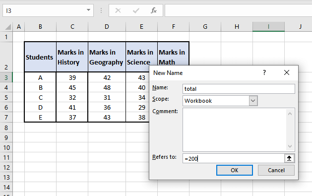
The percentage will be calculated by dividing the sum of the attained marks by the total (each subject is marked out of 50. Which makes 50 x 4 = 200). We will set "200" as our named constant and give it the name "total".

Using "total", we can calculate the percentages without having to refer to "200".

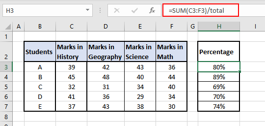
Here, we have substituted "200" for "total" and calculated each student's overall percentage.

How to Make a Named Formula

Taking the above example, what if we named the whole formula and get the same results? Sounds like a good bargain for smart input. Let's see how to do that.

We first head to good old Name Manager and "New Name" again. We will name our formula "Percentage". The reference of this name is shown as

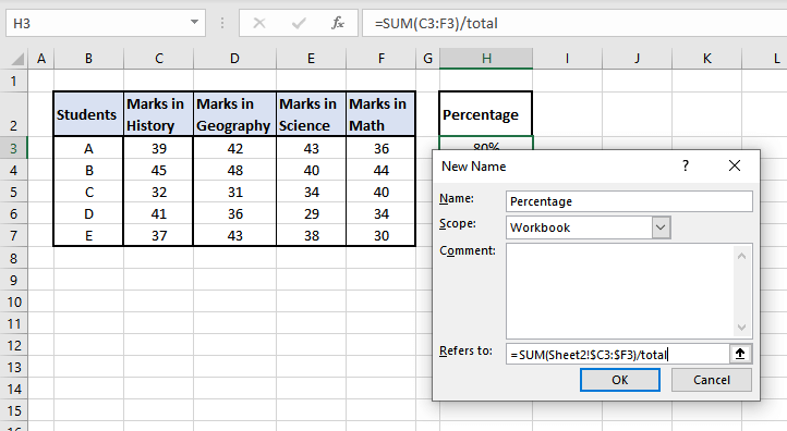
The range of the SUM in the formula is "C3:F3". The columns have been locked into absolute references by the $ sign. Notice that the rows have not been locked as absolute references so that the formula can be dragged to apply to all the rows.

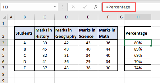
Now just by using "Percentage", we can use the named formula to calculate the students' percentages.

Named Ranges for Data Validation

Named ranges make the "Data Validation" feature in Excel a breeze. You can create a drop-down menu with values from a named range.

This comes with some advantages. You can simply refer to the named range in the Data Validation window instead of having to directly enter the cell ranges. It also gives a point of relevance to see the named range in sight. Let's see how it's done.

Let's assume – we have a list of products and their prices and discounts. Our objective here is to calculate the discounted price for each product after entering its relevant discount. Instead of copy-pasting each discount, we want the option to select the discount from a drop-down menu for each cell in column D.

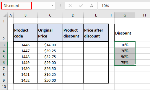
We will create a drop-down menu with the "Discount" named range (G3:G6).

• Select the cells for which you want to create the drop-downs (D3:D9 for our case).

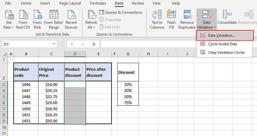
• Under the "Data" tab, in the "Data Tools" section, select "Data Validation" dropdown and click the next "Data Validation" option.
• Inside the "Data Validation" window, under "Allow", choose "List" and enter the required named range under "Source". We will enter the reference of our "Discount" range here.

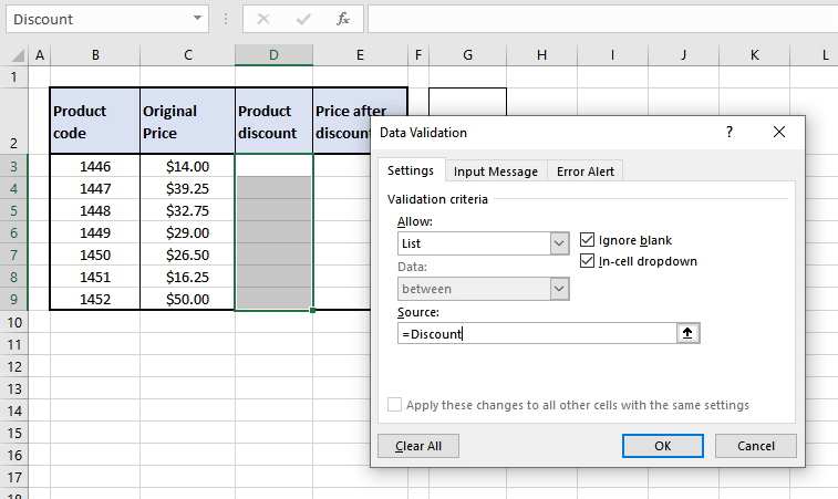
• Click "OK". This has very conveniently created drop-down menus for all cells D3:D9, taking values from the "Discount" named range.

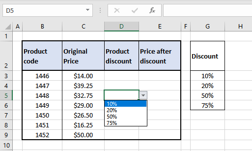
• Now we can select the respective discounts and arrive at our "Price after discount".

See all Names Directly on the Worksheet

There is a small hack that allows you to see all the names directly on the worksheet. You can view all your named ranges (marked with the names) on the sheet if you zoom out to anything less than 40%. We'll follow that religiously and zoom out at 39%.

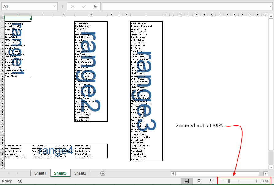
The only thing amiss about this is that the named range text is like a watermark; it's not opaque and will not work so well for small and narrow columns. This hack is suitable for data with a wide-set column or several more rows so the name of the range can be seen. Otherwise, it would be on the brink of being unnoticeable.

Scope of a Name

If you open the Name Manager and have a look at the named ranges, you will find that each named range has a scope (e.g., Sheet1, Sheet2, Workbook, etc.) against it.

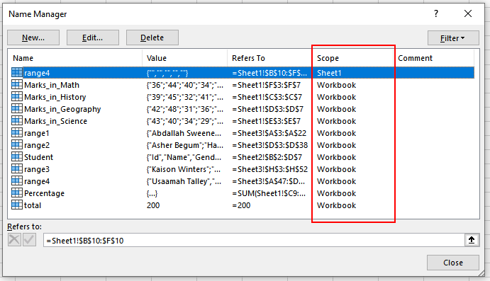
Scope refers to the location, or level, within which the name is recognized. For instance, in the above image "range4" can only be used within Sheet1 whereas all the other names can be used across the entire workbook.

Based on this there can be 2 levels of scopes:

• Local worksheet scope
• Global workbook scope

Local Worksheet Scope

Locally scoped names can only be recognized and used on the sheet it is created upon. This implies that inside a single workbook we can have the same locally scoped names (each within a separate worksheet). For instance – you can have a yearly expense workbook with a worksheet for each month and then we can have a single locally scoped name within each worksheet.

Pro Tip: Named ranges made using the Name Box have global scope by default. However, you can tie the named range down to a sheet (in other words, make it locally scoped) simply by using the sheet's name before the range's name (with an exclamation mark).

Sheet1!Expenses

Global Workbook scope

Globally scoped names can be recognized and used across the whole workbook. Global names must always be unique within the workbook. For instance – we can create a global name to define the value of a constant like pi (as 3.14) and use it across the whole workbook.

Creating Dynamic Named Ranges in Excel

Up until now with all the examples above, we can say that if we were to expand on the data by adding more values, the formulas already applied wouldn't account for the new values. This means that whenever values will be added to the dataset of the named range (e.g., B2:B15) which expands the dataset to B2:B20, the named range will still not account for the additional 5 values and remain a named range for B2:B15. This means the named range is static as opposed to a dynamic named range. The additional step that would need to be taken to fix this is to edit the named range and modify the range mentioned.

A dynamic named range on the contrary will itself adjust for changes in the range. To make our named range dynamic, we will add a function to the reference of the named range. If this sounds too complicated, let us show you how it's done.

There are a couple of ways of creating a dynamic named range. One of them is using the OFFSET function. The drawback is however that OFFSET is a volatile function; with each and every change in a worksheet, OFFSET recalculates. This is not an issue for an uncomplicated worksheet with small datasets. But with complex and large worksheets, you will find that OFFSET slows things down. In such a case, the other way to create a dynamic named range is using the INDEX function.

So if you can use OFFSET for small datasets and INDEX for large ones, why not just master the INDEX function and use that? So this use of the INDEX function for dynamic named ranges is what we'll be tapping into right now. Let's see an example:

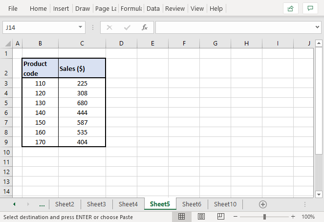
Taking simple sales data, we will add a dynamic named range that we will later use to calculate the total sales:

• Open the "Name Manager" > click the "New Name" option.
• Set the desired name (we are naming our named range "Sales").

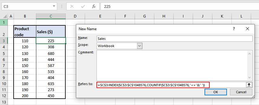
• In "Refers to", feed the following formula, and click "OK".

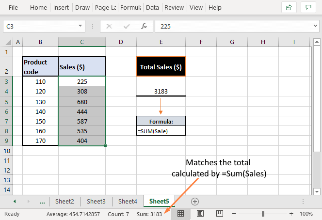
We have used the SUM function to total the named range "Sales". It has given us a total of "3186" which is also confirmed from selecting the cells with the results displayed in the status bar below.

Now let's add some values to this dataset to see if the formula applied complies with changes in the data.

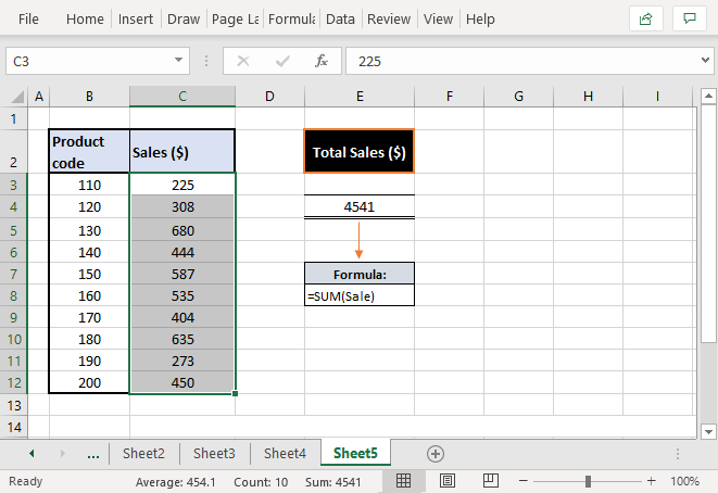
We have added new sales data and the named range has updated itself because of the formula we have put in to build the range. So how does this formula work?

Let's see the formula again:

Since we're using the INDEX function in the formula, let's get familiar with it. The INDEX function returns a value or cell reference of a particular cell in a given range. The part we need to work with right now is the return of a cell reference.

The COUNTIF function counts the number of cells within a range that meets the given condition. The range given to COUNTIF is C3:C1048576. COUNTIF needs to look through the entire C column ahead of C3 (if you press Ctrl + down key, you will find the last row given in Excel which is row number 1048576. That is why we have used C1048576 in our formula. According to how big or small your data is, you can refer to any row ahead of your last value, suppose 100 rows ahead of your last value. In this way the formula will account for all changes made up to the last-mentioned row).

The condition given to COUNTIF is counting the number of cells from C3 to C1048576 that should not be equal to (defined by "<>") blank cells (defined by " "). Take note that this will work only if the data does not consist of blank cells as the blank cells are the ones to be ignored by the function.

According to this condition, the non-blank cells that COUNTIF was able to find from the given range were C3:C9. Passing this result to the INDEX function, INDEX then returns the value of the last item of the list (which would be C9's value i.e., 404). The formula starts with the first cell that we need to include in our named range (i.e. C3, fed as an absolute reference by "$" signs). Using this reference before the INDEX function makes INDEX return the cell reference instead of the value which will then be C9.

The result of the whole formula has worked like this:

Note: Dynamic named ranges aren't shown in the Name Box. Use the Name Manager to see all named ranges (static and dynamic).

Named Range Shortcuts

The more matters are sitting on your fingertips, the better. To wrap things up, here are some useful keyboard shortcuts with named ranges that should move you around the sheet even faster.

• F3 – Pops up a "Paste Name" dialogue box for pasting a named range from the full list of named ranges.
• Ctrl + F3 – Opens "Name Manager"
• Ctrl + alt + F3 – Pops up "New Name" dialog box for creating a new named range.
• Ctrl + shift + F3 – Pops up "Create Names from Selection" dialog box for creating named ranges from headings/titles.
• F5 – Pops up the "Go To" dialog box for navigating to the chosen named range from the full list of named ranges.

With that, we've discussed the ins and outs of the Named Ranges in Excel. They are simple, but extremely useful while working with larger datasets and multiple ranges. While you solidify your expertise with some practice, we'll have another awesome tutorial ready for you ready!