Organizing is good but sometimes a measure of randomness makes things better. That is true for life and Excel and we are here for the Excel side of matters. Excel is quite proficient with sorting lists; alphabetical order, chronological order, ascending and descending order but it’s yet to come up with straight-up randomization (nearly oxymoron-ish). Although we do have functions to help us along with that and that’s what we will be looking up in a bit.
You may want to randomize a list of names of students, employees, contestants, etc. just to prevent tipping the balance that comes from good old alphabetical sorting. You might want to rearrange dates or scramble a list of names or products. Or maybe you’re just randomly aiming to be an Excel nerd.
This tutorial will teach you how to randomize a list in Excel using functions alone and also with the Excel Sort & Filter feature. While we’re at it, you’ll also learn to use functions to make a random pick from the list.

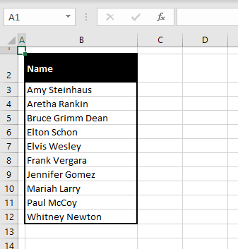
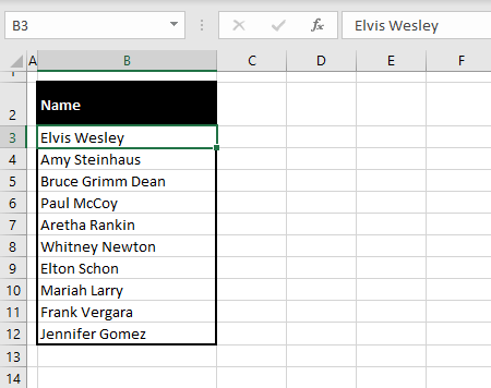
For our example to be used throughout this guide, we will randomize the following list of names that are arranged in an alphabetical order:
Let’s start exploring the options and see what we can do to randomize lists.
Method #1 – Using RAND Function & Sort Feature
We can’t randomly sort names but we can have an arrangement of random numbers. This is where we will utilize the RAND function. The RAND function returns a random number greater than 0 and less than 1. We will get a list of random numbers lined up with the names and then sort them using the Sort & Filter tool which will then have the names randomly scrambled. Let us show you the steps.
- Enter the RAND function against the first name in a new column. This is the formula you need to enter:
=RAND()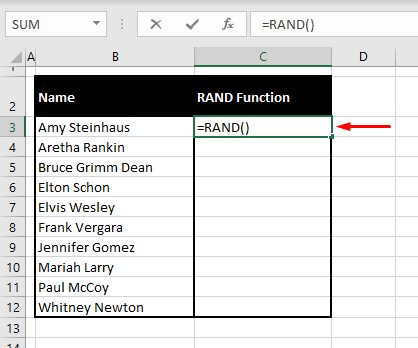
- This formula is simply the RAND function applied on its own with no arguments. The RAND function returns random values that are greater than 0 but less than 1.
- Select and drag the formula.
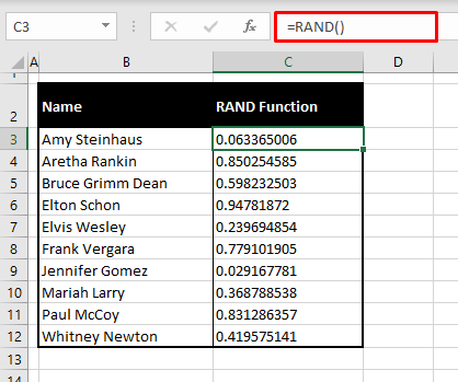
- Select any cell containing the number. Navigate to the Home tab > Editing group, select the Sort & Filter option. From the drop-down, select either of the top two options. We will go with the first one – Sort Smallest to Largest.
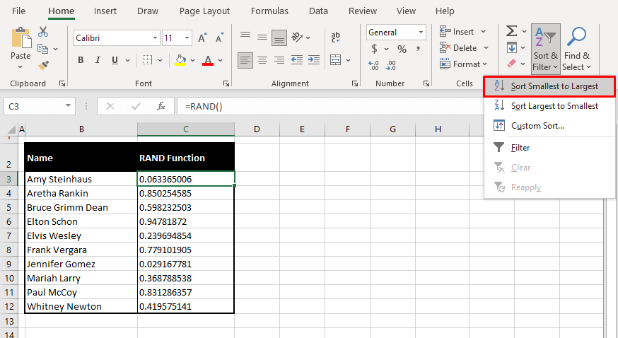
- This will rearrange the names to be randomly jumbled. The numbers will recalculate (which is a part of random functions) and not to worry, since you won’t be needing them much longer.
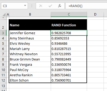
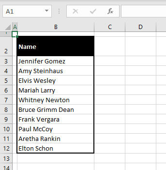
- Now that we have our random list ready, we can select the column with the RAND function and delete it.
Notes:
We mentioned in the steps that recalculation of the numbers is a part of random functions. By that, we mean the RAND is a volatile function and for all volatile functions, Excel triggers recalculation on every worksheet change. This means you can keep scrambling the data (names in this case) using the Sort & Filter tool until the randomness is good to go.
The data in any columns aligned with the RAND function column will also rearrange linearly. Even if there are columns on both sides of the RAND function column, they will all rearrange linearly together.
The upside of this method is that you keep the original list and randomize that instead of creating a new list from the original as a base.
Method #2 – Using RANDBETWEEN Function & Sort Feature
Not very different from the method above – we’re only switching things up here, swapping the RAND function for the RANDBETWEEN function. The RANDBETWEEN function returns a random number between the specified range.
First, we will use the RANDBETWEEN function to return random numbers against our list of names. Then, we will use the Sort & Filter tool to rearrange those random numbers, which will also rearrange our list of names into a randomized list. We have the steps as follows:
- In the column next to the names, enter the following formula for the RANDBETWEEN function:
=RANDBETWEEN(1,10)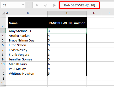
- In this formula, we use the RANDBETWEEN function to return a random number from 1 to 10.
- Select any cell from the range and navigate to the Home tab > Editing group > Sort & Filter button > Sort Smallest to Largest (any of the two options will work).
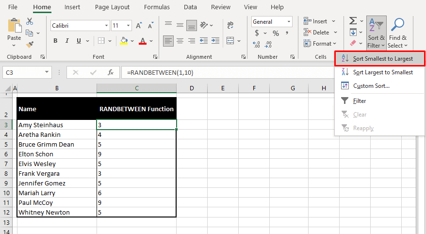
- This will rearrange the names to be randomly jumbled. The numbers will recalculate (RANDBETWEEN too is a volatile function) which is not an issue since you will be deleting the numbers soon.
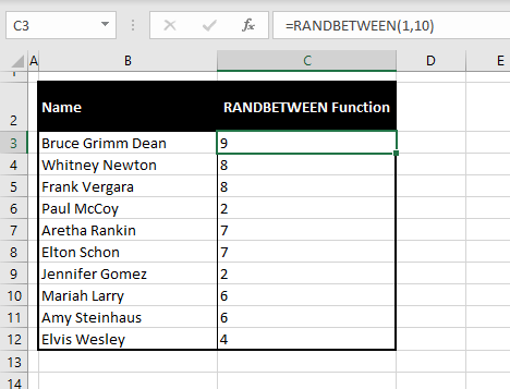
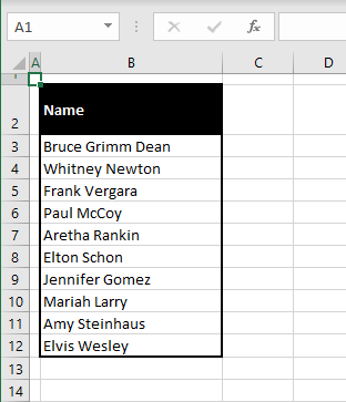
- Now that we have our random list ready, we can select the column with the RANDBETWEEN function and delete it.
Method #3 – Using RANDARRAY, SORTBY, & ROWS Functions
Using a base list, a randomized list can be created using the RANDARRAY, SORTBY, and ROWS Functions. The RANDARRAY function returns an array of random numbers. The SORTBY function sorts a range based on the values in a corresponding range. The ROWS function returns the number of rows in a reference.
For the formula we will use, the ROWS function will return the number of rows for RANDARRAY to randomize. Then the SORTBY function will sort the list according to the randomized rows.
Let’s see how all of this looks on a sheet. Enter the following formula in a separate column:
=SORTBY(B3:B12,RANDARRAY(ROWS(B3:B12)))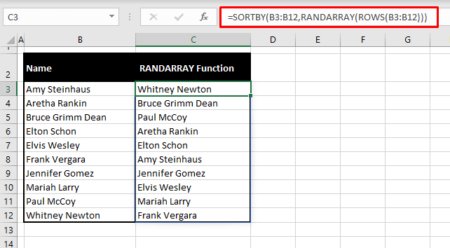
The ROW function returns the number of rows in B3:B12 which is 10. The RANDARRAY function takes that number and returns an array of 10 random numbers for all 10 rows. Then the SORTBY function sorts B3:B12 according to the randomized numbers which randomly adjusts B3:12 into a new list.
This is quite like the two methods above without having a separate column for random numbers.
There is no need to make the list of names into absolute references in the formula. There is also no need to drag the formula since the results of this formula spill to create the randomized list.
Select the new randomized column, and copy-paste the values on themselves or in a new column to avoid #REF errors when the original column is deleted. Delete rest of the data which is not needed anymore.
All three methods mentioned up until now are good if you do not want to duplicate values in your finished randomized list.
Recommended Reading: How to count non-blank cells from a list
Method #4 – Using INDEX and RANDBETWEEN Functions
A randomized list can be created using the INDEX and RANDBETWEEN functions. Before you decide to proceed with this method, there will most probably be a repetition of values (repetitions of names in this case). If that is not an issue, let’s continue.
The INDEX function returns a value or its cell reference at the intersection of a particular row and column in a given range. The RANDBETWEEN function returns a random number between the specified range. In our formula, the INDEX function will work to return the value of the cell that RANDBETWEEN randomly specifies.
Let’s crack on with the sheets. Enter the following formula in a separate column:
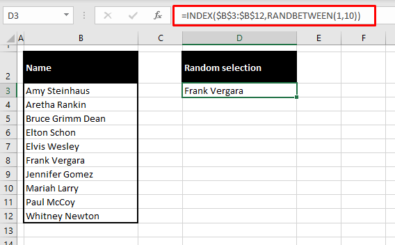
=INDEX($B$3:$B$12,RANDBETWEEN(1,10),1)You can use this formula for a single selection:
Or you can drag the formula for a randomized list:
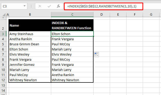
The RANDBETWEEN function randomly returns a number from 1 to 10. In the first case, the random number generated is 4. This result is fed to the INDEX function in place of a row number. This means that the INDEX function is set to return the 4th value from the range B3:B12 which in the first instance is “Elton Schon”.
“1” at the end of the formula is not really required here but is useful if the range-fed into the formula is for a table (multiple columns) instead of a list (single column). This number signifies the column number from which the result is to be picked.
The formula has been dragged to fill the rest of the column.
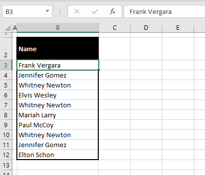
Select the new randomized column, and copy-paste the values on themselves or in a new column to stop the column values from recalculating. Delete the rest of the data not needed anymore.
Notes:
For randomizing a list this way, the values will repeat. That is because of the nature of the RANDBETWEEN function randomly returning a number from the specified range. This way, each result is mutually exclusive and so the numbers can (and do) repeat.
There are a few tweaks that you can make using the RANDBETWEEN function for a randomized list without duplicates, adding more functions into the works but that would make the process lengthier and unnecessarily complicated when there are other methods that get the work done in much simpler ways. If repetitions are not an issue, then this method is alright to go with and is well suited for a single random pick too.
Also, since RANDBETWEEN function is a volatile function so its value gets recalculated on every worksheet change. This means you can keep scrambling the data (names in this case) until the randomness is good to go.
Method #5 – Using CHOOSE and RANDBETWEEN Functions
Similar to the above method we can also generate a randomized list using the CHOOSE and RANDBETWEEN functions. A heads-up on this method; the results (names in this case) are most likely to repeat.
If that’s alright, then keep reading.
The CHOOSE function chooses a value from a list of values based on an index number. The RANDBETWEEN function returns a random number between the specified range. In our formula, the CHOOSE function will choose a name from the list of names according to the number that RANDBETWEEN randomly specifies.
Time for working the sheets. Enter the following formula in a separate column:
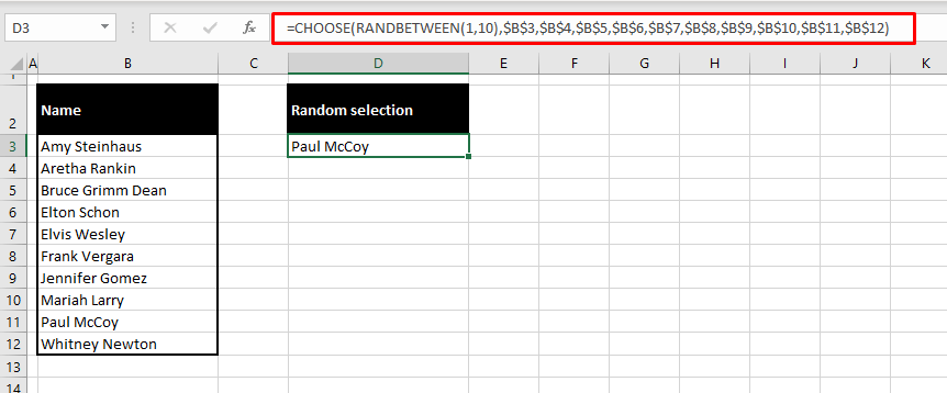
=CHOOSE(RANDBETWEEN(1,10),$B$3,$B$4,$B$5,$B$6,$B$7,$B$8,$B$9,$B$10,$B$11,$B$12)You can use this formula for a single selection:
Or you can drag the formula for a randomized list:
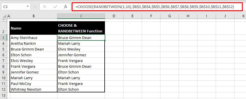
The RANDBETWEEN function randomly returns a number from 1 to 10. In the first instance, the random number generated 3. The CHOOSE function then selects the 3rd value from the list of values fed into the function. The final result is “Bruce Grimm Dean”.
The formula has been dragged to fill the rest of the column. The list's cell references are entered as absolute references in the formula so that the references don’t change as the formula is dragged.
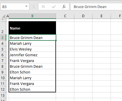
Select the new randomized column, and copy-paste the values on themselves or in a new column to stop the column values from recalculating. Delete the rest of the data which is not needed anymore.
Notes:
Similar to the INDEX and RANDBETWEEN method, this method also can cause the values to repeat because of the nature of the RANDBETWEEN function. So make sure to only use it when having repetitions in the list is not an issue.
Here we come to a not-so-random end of this tutorial. We hope to have delved enough into the ways of randomizing a list in Excel to give you a good grasp of what works for your Excel situation. We will be back with more how-tos and all-about on everything in Excel. Feel free to come back for more problem-solving!

