How to Square a Number in Excel (5 Quick & Easy Ways)

The aim is simple. Squaring a number, a number raised to the power 2, the number multiplied by itself; it's all the same thing, you know the drill. If this is giving you unfond memories of your childhood math classes, it's a good thing you're here because we aren't going to math-splain you.

This tutorial is about squaring a number in Excel, and we will break down all the methods mentioned above. Throughout this tutorial, for our examples, we will square the numbers in one column and try to print the results next to them using different easy peasy ways.

Let's start diving into the easy peasy ways which we will split into 2 sections; in the first section, we will square numbers using formulas and in the second section, we will use functions.

Squaring Numbers Using Formulas

In this section, we will use two formulas to square numbers:

• Formula using multiplication operator
• Formula using caret operator

Let's see them one by one.

Method #1 – Using Multiplication Operator

By multiplication operator, we are referring to the asterisk ( * ) symbol. A squared number is basically the number multiplied by itself so we will do just that on our worksheet in the form of a formula. Let's see this practically.

We will use the following formula in our example:

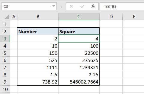
This reads as B3 multiplied by B3. The value in cell B3 is 2 and so the calculation goes as 2 multiplied by 2. Here is the outcome:

Also, instead of making use of the cell references, you can apply the formula directly as:

Wasn't that easy breezy? It's nice to have Excel do all the work for you. Let's keep flowing with the easy breeze into the next formula.

Method #2 – Using Caret Operator

By caret operator, we are referring to the " ^ " symbol. Caret Operator is also known as Exponent operator. Does anyone remember five raised to the power two?

(Hint: Math classes again)

The caret is essentially saying 'raised to the power'. Hence, 5 raised to the power 2 becomes 5^2, squaring the number 5. Let's see how it helps us in Excel.

Referring to our example, the formula using the caret symbol to square a number will be:

This reads as B3 raised to the power 2. The value in cell B3 is 2 and so the calculation goes as 2 raised to the power 2 with "4" as the squared result. Applying this formula to square numbers will give us the following results:

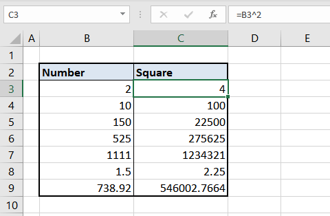
Also, instead of relying on the cell references, you can apply the formula directly as:

Just now, we used a formula to raise the power of a number. We can apply the same principle using a function, which brings us to our next section where we square numbers using functions.

Recommended Reading: Calculate Square Root of a Number

Squaring Numbers Using Excel Functions

This section covers the use of functions to square numbers. The functions we will use are:

• The POWER function
• The PRODUCT function
• The SUMPRODUCT function

Method #3 – Using POWER Function

The POWER function works like a caret operator, raising the number to a power. The syntax of POWER function is very simple it takes two arguments: number and power.

For the purpose of this article, we are interested in squaring the number so we are working only with raising the numbers to the power "2". The POWER function can easily do that for us.

This is how we will use the POWER function for our example:

The value in cell B4 is "10". The "2" in the second argument here is the power by which the number in cell B4 ("10") is to be raised. The result of 10 raised to the power 2 is 100 which we have in our results:

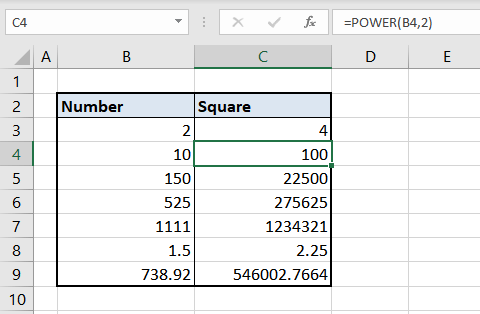
For instances where you wish to skip the cell reference in the function, you can apply the function directly as:

Method #4 – Using PRODUCT Function

The PRODUCT function will multiply all the numbers given as arguments. Similar to how we used a multiplication formula to multiply the number with itself, we can use the PRODUCT function for the same calculation, separating the numbers by commas instead of asterisks (*).

Carrying down our base example, for squaring a number, we will need to supply the number twice in the formula and that should do it:

Cell B4 contains the number "10". Since the PRODUCT function multiplies all the supplied numbers, for squaring the number 10, we only need to supply it twice to the formula. 10 multiplied by 10 gives us 100 which we also have here in the results:

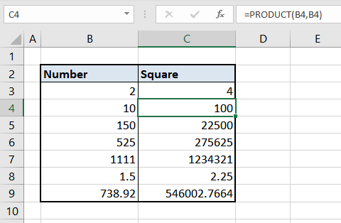
For instances where you wish to skip the cell reference in the function, you can apply the function directly as

Similar to the PRODUCT function, we can use the SUMPRODUCT function for squaring numbers. Let's see ahead.

Method #5 – Using SUMPRODUCT Function

An extension of the PRODUCT function, the SUMPRODUCT function multiplies the supplied number groups and then adds the outcomes of the multiplied groups for the final result. It works like this:

For instance, if we have a SUMPRODUCT function as:

Then the result will be calculated as  –

The SUMPRODUCT function will multiply each element from both the cell ranges and then added them to one another to return the final result.

Mathematically this is equivalent to writing –

(A1*B1) + (A2*B2) + (A3*B3)

Now, lets jump back to our case –

For squaring a number we need to multiply the number by itself. Therefore, we only need to pass one group of numbers to the SUMPRODUCT function. SUMPRODUCT will multiply that for us and hand us the result. We are to use it just like the PRODUCT function.

So if we are to use it exactly like the PRODUCT function, why add the "SUM" prefix? Well, since we are exploring options and this is viable, we have to have the talk about it. Let's put it to use with our example.

Cell B4 contains the number "10". As the SUMPRODUCT function multiplies all the supplied number groups and then adds the result of those multiplied groups, we will only provide one number group i.e. "B4, B4" which will be "10, 10" since that is what we require for squaring the number.

SUMPRODUCT will multiply 10 by 10. The result will be 100. Since there is no other number group to multiply, the final outcome of SUMPRODUCT is 100.

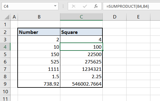
For instances where you wish to skip the cell reference in the function, you can apply the function directly as:

This ends our tutorial, fair and square. Thanks to the power of Excel, we have many options for the simplest of calculations. There's so much more to explore and this is just a wodge of Excel. We'll come up with another wodge soon, be sure to have your part!