In the last article, we worked with the DATVALUE function to convert dates from text to a serial number. Now let’s take things up a notch and look at some formulas that will enable us to manipulate dates and times in a worksheet.
In this tutorial, we will try to understand how to subtract dates in Excel and calculate the difference between dates and times. So, without further ado, let's get straight into the topic.

Get Number of Days Between Two Dates
Subtracting two dates in Excel gives you the number of days between those dates. It is quite simple to accomplish, of course. If you have readily formatted dates in any two cells, just subtract those cells. For example:
=B2-A2 //EndDate - StartDate
The formula has a straightforward process. It takes both dates (from cell B2 and A2), and subtracts them to compute the number of days in between, i.e. 584 days in our example. Make sure that the output cell is not formatted as a date, though.
Similar, results can also be obtained by using the DAYS function. To calculate the number of days between two dates, days function can be used as –
=DAYS(B3,A3) //where B3 is the EndDate and A3 is the StartDateIf you have a list of dates that you would like to subtract from today's date, you may use the following formula:
=TODAY()-A4
Using TODAY() in the formula will instruct Excel to refer to your system’s current date while running the computation. Note that this formula will give you a different answer as the date keeps changing, which means it will update your output automatically every day, i.e. your output will increase by 1 every day.
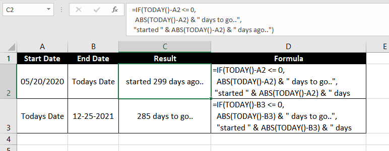
But this formula has a problem, it will return negative numbers if A4 has a value greater than today's date. To solve this we can make use of the IF Function and create a formula that gives a more descriptive result.

=IF(TODAY()-A2 <= 0, ABS(TODAY()-A2) & " days to go..", "started " & ABS(TODAY()-A2) & " days ago..")Get Years, Months, and Days Between Two Dates
This is where things begin to spiral ever so slightly into complexity. We will walk you through the formulas—fasten your seat belts.
Here are the formulas we will use:
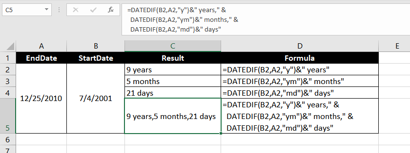
=DATEDIF(B2, A2, "y") & "years" //Gets Year part
=DATEDIF(B2, A2, "ym") & "months" //Gets Month part (days and years are ignored)
=DATEDIF(B2, A2, "md") & "days" //Gets Day part (months and years are ignored)
The DATEDIF function has three arguments. The first and second arguments are pretty straightforward, those are the dates you want to subtract. Ensure that the date in the first argument falls before the date in the second argument; otherwise, the formula will return a #NUM! error.
The third argument tells the formula whether you want to subtract the days, months, or the years ("y" for years, "ym" for months, and "md" for days).
Also, if you want to subtract all three components, you can add a concatenation operator ("&") between these formulas to return all three components as shown in the picture, like so:
=DATEDIF(B2,A2,"y")&" years," & DATEDIF(B2,A2,"ym")&" months," & DATEDIF(B2,A2,"md")&" days"Adding a concatenation operator allows us to display the output from these 3 formulas in a single cell.
First, the formula computes years and adds the string " years," which gives us the output "9 years" in our example. The second formula computes months and adds the string " months," to give us the output "5 months," and the third formula returns "21 days".
When you add a concatenation operator between these formulas, all the returned strings are displayed in a single cell giving us our final output "9 years, 5 months, 21 days".
Get Difference Between Two Dates (with Time) in Hours
Before we get into these computations, it is important to know how Excel interprets time. Again, Excel likes to work with numbers. Just like it assigns a serial number for a date, it assigns a fraction for time. For example, 0.25 is 6 am and 0.5 is noon (or half a day).
Subtracting 2 cells containing date and time is a straightforward process, but the formula looks moderately long because of the mechanics involved for a polished outcome. Here is the formula we will use:
=INT((A2 – B2) * 24) & " hours" //where A2 is EndDate and B2 is the StartDate
Upon subtraction, we get a fraction. Here is how Excel computes this return: (Number of days between both dates + a fraction for the difference in the number of hours).
Let’s work out these numbers to see what is cooking inside the formula.
What’s happening inside the brackets…
The total difference between both times is 24 hours, 30 minutes, 25 seconds. Excel will first compute the difference in terms of days, and return 1 day (i.e. 24 hours). This leaves out the 30 minutes and 25 seconds, which still need to be factored into the output. Since our time is mentioned down to the seconds, we will compute 30 minutes and 25 seconds in terms of total seconds, like so:
- 30 minutes * 60 seconds/minute = 1800 seconds
- 25 seconds
The total seconds, therefore, are 1825 seconds. To compute the fraction, we will divide 1825 seconds by 86,400 seconds (i.e. the total number of seconds in 1 day).
The fraction that we get, as a result, will naturally be in terms of days and can be directly added to the 1 day we computed earlier. The fraction we get by dividing (1825/86400) is 0.021122.
Great, so the final difference between our 2 DateTimes is (1 + 0.02112 days) or 1.02112 days.
Exiting the brackets
Outside the bracket, we are multiplying the output by 24.
Why?
Well, we want our final output in hours, right? If our current output is in terms of days, multiplying it by 24 will convert it to hours. That will give us (24 * 1.02112) 24.507 hours.
Now, you could get away with just the bare-bones formula nested inside the INT function, and you will still receive pretty much the same output without adding the text string at the end. As I said, the INT function removes decimals so the return (24 hours) looks more pleasant to the eye.
Get Difference Between Two Dates (with Time) in Minutes
Not a lot of difference here, naturally. The only difference will be that instead of 24, you will multiply 1440 in the formula, and replace the text string with the word "minutes" like so:
=INT((A2 - B2) * 1440) &" minutes" //where A2 is EndDate and B2 is the StartDate
The formula works the same way as discussed in the previous example. The only difference is instead of multiplying the bracket with 24, we multiply it with 1440 (i.e. total number of minutes in a day) since we want our output in terms of minutes.
Get Difference Between Two Dates (with Time) in Seconds
Ah, you guessed it!
The only difference, again, will be that we will multiply 86400 inside the formula, and use the text string "seconds" like so:
=INT((A2 - B2) * 86400) &" seconds" //where A2 is EndDate and B2 is the StartDate
Again, the formula works the same way. This time around, we multiply the bracket with 86400 (i.e. total number of seconds in a day) since we want our final output in terms of seconds.
Get Days, Hours, Minutes, and Seconds Between Two Dates (with Time)
Now, let's take it one more step further and try to fetch the difference between two dates in terms of days, hours, minutes, and seconds. To do this we can use the following formula –
=INT(A2 - B2) & " days, "& TEXT(A2 - B2,"h"" hours, ""m"" minutes, ""s"" seconds""") //where A2 is EndDate and B2 is the StartDate

Okay, this may look like a Frankenstein formula, but it is quite the opposite.
A large portion of work is being done by the TEXT function here. Using the TEXT function, we are applying a custom number format (that we generally apply using the "Format Cells" dialog box) to the output generated by subtracting both the dates. The TEXT function takes care of the hours, minutes, and seconds in our final output.
For days, we use the INT function, which is just the integer of the return generated by subtracting both the dates.
Finally, we tie both the INT and TEXT functions together with a concatenation operator to get our final output, i.e. 1 days, 2 hours, 30 minutes, 25 seconds.
Subtracting Two Times (Without Date) to Find the Difference
Quite intuitively, this is only possible for computations that do not exceed 24 hours. For computations exceeding 24 hours, look at the "subtract DateTime from another DateTime" section.
There are no separate formulas required here. All we need to do is subtract the two cells, like so:
=A2 – B2 //where A2 is EndDate and B2 is the StartDate
The only important thing to look at here is the format of the output cell. You must use a custom format "h:mm:ss" for the output to appear correctly.
Alternatively, you could use the TEXT function to apply a custom number format to the output, using the following formula:
=TEXT(A2 - B2, "h:mm:ss") //where A2 is EndDate and B2 is the StartDate
Notice how we are still subtracting A2 from B2 in this formula. The ONLY difference here is that instead of applying a custom number format manually, we use the TEXT function to apply the "h:mm:ss" format to the output.
Subtracting Hours, Minutes, or Seconds from a DateTime
Before we dive into these computations, note that the TIME function can really simplify subtracting time for us, but it has a limitation. It allows subtraction of a maximum of 23 hours, or 59 minutes/seconds only. So, we will use some workarounds and construct a formula.
Subtract Hours from a DateTime
Let’s say we have a particular date and time and we want to compute a date and time that was a certain number of hours before. We will use the following formula for our computation:
=A2 - (hours to be subtracted / 24) //where A2 contains the DateTime
It is a simple computation where we want to go back 30 hours in time from December 25, 2001 midnight. However, Excel makes date computations in terms of days. So, we must give Excel the number of days we want to subtract from the date in cell A2. To do this, we just divide 30 by 24.
So, how does Excel compute the time then?
Well, notice that dividing 30 by 24 will give you 1.25 days. Here, the numbers after the decimal represent time, while the number before the decimal represents days.
Excel will subtract 1 day and (0.25 * 24 = 6) hours from the date in A2 because Excel thinks of time in terms of fraction/decimal.
Our return in this case, of course, is December 23, 2001, 6:00 pm.
While the formula mentioned above works in all cases, we can also use the following formula if the hours to be subtracted are less than or equal to 23:
=A2 – TIME (20, 0, 0)Subtract Minutes from a DateTime
We will use the same formula that we used for subtracting hours for subtracting minutes, with the only change being the denominator in the formula:
=A2 - (minutes to be subtracted / 1440) //where A2 contains the DateTime
Much like the previous example, we enter the number of minutes we want to subtract in the formula’s numerator, which is 3500 minutes in our case. In the denominator, we will use the total number of minutes in 1 day (24 hours * 60 minutes = 1440) to convert the value in the brackets to days from minutes. The remainder of the logic remains the same as the previous formula.
This gives us December 22, 2001, 2:10 pm.
Subtract Seconds from a DateTime
Exactly — no change. The formula remains the same except for the denominator in the bracket:
=A2 - (seconds to be subtracted / 86400) //where A2 contains the DateTime
Again, to convert seconds to days, we will divide the numerator by the number of seconds in a day (24 hours * 60 minutes * 60 seconds = 86400).
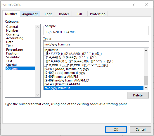
However, note that in order to display date and time in the m/d/yyyy h:mm:ss format, you will need to custom format the cell, like so:

That is all you need to learn about playing around with dates and times on your worksheet. Spend a little time with them, and by the time you ace these formulas, we will be back with more. Until then, keep crunching those numbers!


