Few weeks back, one of my regular visitors dropped me an email describing an issue that he was facing. His task was to add the contents of certain cells based on their background colors.
As we all know, Excel by default has no formula or feature to calculate such a thing. So, in this post I will share few methods that will help you to achieve this.
To make the task more clear let’s have a look at the below image.
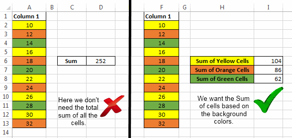
This image depicts that here we don’t need the total sum of all the elements but instead we want the sum of elements that have the same background color.
Recommended Reading: Weighted SUM in Excel
Method 1: SUM cells on the basis of background colour using SUMIF Formula:
We know that SUMIF function is a combination of SUM and IF formula and hence SUMIF can come quite handy for adding cells based on color.
If you don’t know how to use a SUMIF Function, then before going any further I would strongly suggest you to read this post.
First of all let’s try to understand how we are going to do this:
Consider we have a table as shown in the below image.
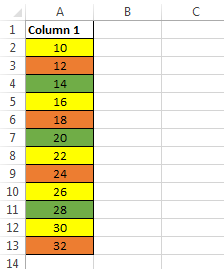
Next, we will add one more column to this table where we will manually type the background colors of their adjacent cells as shown in the below image.
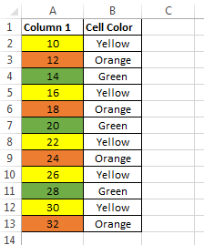
Now, we try to use SUMIF Formula for finding the SUM of cells with yellow background as:
"Yellow",A2:A13)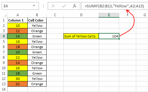
Similarly, for finding the SUM of Orange and Green background cells we will use the formulas
"Orange",A2:A13)and
=SUMIF(B2:B13,
"Green",A2:A13)respectively.
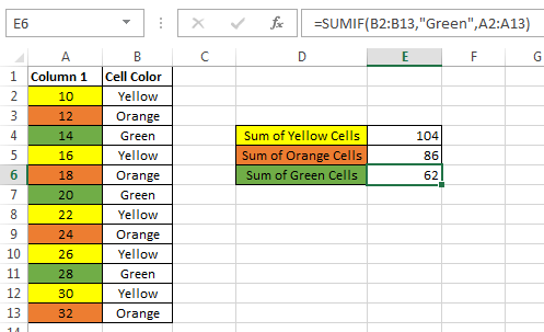
But, as we can see that this method is quite cumbersome, particularly if we need to use this on lists with hundreds of elements.
So, what’s the faster alternative?
To make the above process easier to use we need to reduce the effort of writing cell background colors manually.
So, for this task we can use a small user defined function (UDF) which will do the trick for us.
Function ColorIndex(CellColor As Range)
 ColorIndex = CellColor.Interior.ColorIndex
End Function
Note: This function does not return the color name but it returns the color index which is also a unique value and can be used in our task.
Follow the below steps to use the UDF:
- First of all open your worksheet where you need to add the cells based on background colors.
- Next, press ALT + F11 to open the VB Editor. Navigate to ‘Insert’ > ‘Module’.
- After this, paste the “ColorIndex” UDF in the Editor.
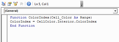
- Now, add one column next to the range that you wish to sum up. In this new column enter the formula as:
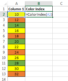
- After that, drag this formula to the whole range.
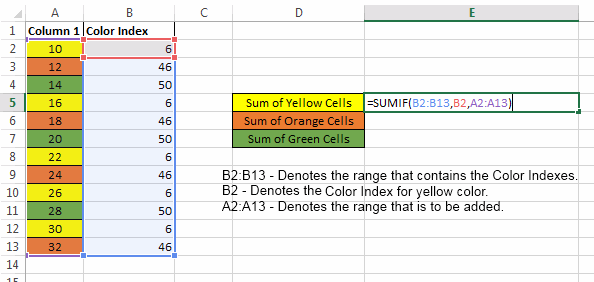
- Now, you can use the SUMIF function to add the cells that have same background color as shown in the above image.
Method 2 : Using a much faster and better UDF:
The UDF that we are going to use in this method is simply an extension of the above used function.
This Function is as under:
Function SumByColor(CellColor As Range, rRange As Range)
Dim cSum As Double
Dim ColIndex As Integer
ColIndex = CellColor.Interior.ColorIndex
For Each cl In rRange
 If cl.Interior.ColorIndex = ColIndex Then
 cSum = WorksheetFunction.Sum(cl, cSum)
 End If
Next cl
SumByColor = cSum
End Function
How to use this UDF:
Follow the below steps to use this Function:
- Open your target worksheet.
- Press ALT + F11 to open the VBA Editor and navigate to ‘Insert’ > ‘Module’.
- Paste the “SumByColor” Function in the Editor.
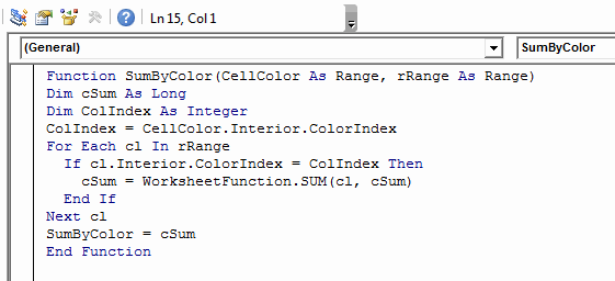
- Now, simply type the “SumByColor” function to call it and pass the following arguments:
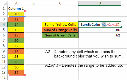
Note:In the formula shown in above image instead of the first argument “A2” we could have also used any one of A2, A5, A8, A10, A12. Because all these cells have yellow background.
In our case we can use the following formulas:
- Sum of Yellow Cells:=SumByColor(A2,A2:A13) //As ‘A2’ is the address of yellow cell and A2: A13 is the range to be added
- Sum of Orange Cells:=SumByColor(A3,A2:A13) //As ‘A3’ is the address of orange cell and A2: A13 is the range to be added
- Sum of Green Cells:=SumByColor(A4,A2:A13) //As ‘A4’ is the address of green cell and A2: A13 is the range to be added
So, this was all from me about this topic. Don’t forget to get the sample spreadsheet [link] and do let me know in case you face any issues while using these methods.


